From decay to date: radiocarbon dating in BraDypUS 5

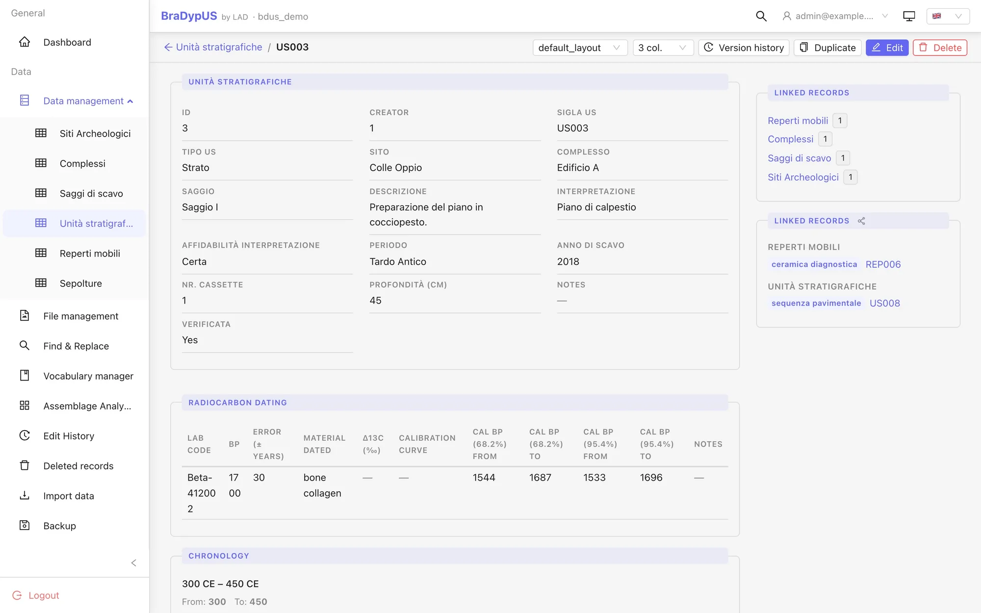
In the previous article of this series, Dating the uncertain: the chronology system of BraDypUS 5, we described fuzzy_date: the plugin that records interpreted datings — the ones an archaeologist writes down based on stratigraphy, materials, typological comparisons. We closed that article with a question left open: what about scientific dates, the ones that come out of a lab rather than out of reasoning? This article is the answer: the radiocarbon plugin, which records radiocarbon (C14) determinations and automatically calibrates them into calendar years.

Before getting into it, a premise that holds for the whole article: radiocarbon is an experimental plugin. It shipped with v5.3.0, only one calibration curve is currently supported (IntCal20), and several features are deliberately left out — we list all of them further down. Development continues based on reports and requests from people using it in the field: the official documentation is at docs.bdus.lad-sapienza.it/guide/system-plugins/radiocarbon.html, and it remains the most up-to-date reference for the plugin’s status.

What the radiocarbon plugin does

Activation looks, on the surface, identical to fuzzy_date’s: Config → Tables, select the table, scroll to System plugins, switch on Radiocarbon dating.

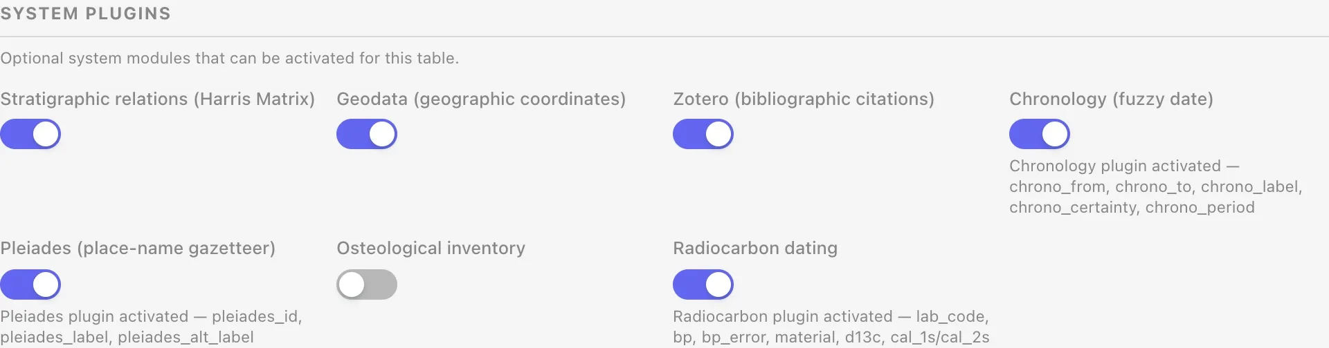The System plugins panel for the Stratigraphic units table: Radiocarbon dating is one of the available system plugins, here activated together with Chronology (fuzzy date) and the others.

Underneath, though, the mechanism is different — and it’s worth explaining, because it isn’t an implementation detail, it changes what you can record. fuzzy_date adds five columns to the table itself: a stratigraphic unit has one interpreted chronology, full stop. Radiocarbon doesn’t work that way — the same context can have zero, one, or several lab determinations (different samples, different materials, occasionally even different labs re-dating the same sample). Activating radiocarbon therefore doesn’t touch the table you activate it on: it creates a dedicated child table, named {table}_radiocarbon (for us it will be us_radiocarbon), one row per determination, linked back to the parent record. It’s the same generic “plugin table” architecture already used for measurements, finds-per-SU, and the like — not a special case.

The child table’s fields:

The four calibrated fields cannot be typed in by hand: whatever value the client sends for cal_1s_from, cal_1s_to, cal_2s_from, cal_2s_to is discarded server-side, and recomputed from scratch on every save from bp and bp_error. This is a deliberate choice, and a different one from how fuzzy_date behaves: there, the client computes the label and the system trusts it; here it doesn’t, because the calibrated range is scientific derived data that feeds search and filters, not a cosmetic label.

Using it, in practice

The record page gains a Radiocarbon dating section, with the same row-based editor already seen for other plugin tables: add a row, fill in lab code, BP, error and material, save.

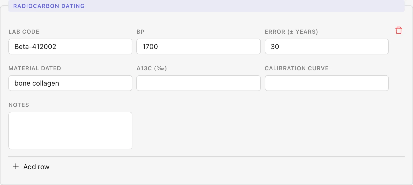The panel in edit mode. The only fields missing are the four Cal BP ones, read-only: everything else — including d13c and curve, still empty here — is editable.

After saving, the record shows the full row, with the calibrated ranges computed by the server:

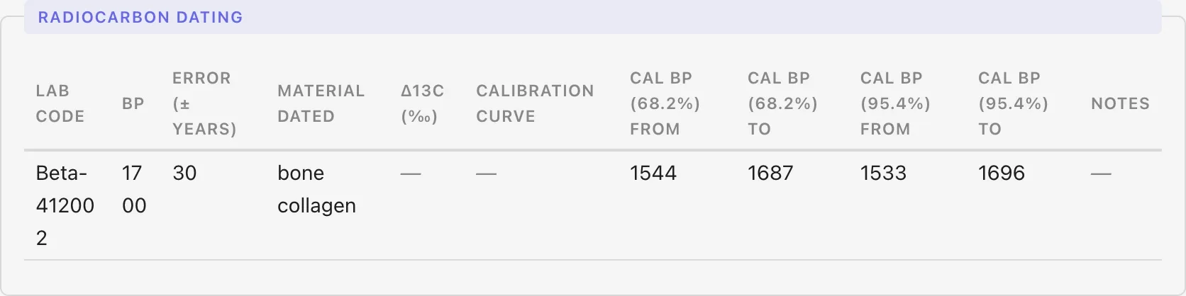The panel in read mode for US003: a determination on bone collagen, BP 1700 ± 30, calibrated to 1544–1687 cal BP (68.2%) and 1533–1696 cal BP (95.4%).

One notational point worth clarifying right away, since it trips up anyone who doesn’t handle it daily: cal BP means “calibrated years before present”, where “present” is conventionally fixed at 1950. To turn it into calendar years, subtract from 1950: the example above, 1544–1687 cal BP, becomes cal AD 263–406. It’s not a coincidence that US003 is catalogued, in the interpreted chronology (fuzzy_date), as “Late Antique”, AD 300–450: the two datings — one scientific, one interpretive — overlap but don’t coincide exactly, and that’s expected: they’re two independent lines of evidence, not a copy of one another.

As with fuzzy_date, deactivating the plugin is a configuration action, not a deletion: radiocarbon disappears from the table’s visible plugins, but the child table and its rows stay intact, ready to reappear if you reactivate it. To actually delete the data, today, the only route is to drop the {table}_radiocarbon table from Config → Tables like any other table — an irreversible action, and one the UI flags clearly as such.

Technical appendix: how the calibration works

This section is for readers who want to see the algorithm, not just the result. The code lives in lib/Radiocarbon/Calibrator.php (readable on GitHub): a static class, no I/O, that takes bp, bp_error and a curve name, and returns two pairs of integers.

The curve itself — lib/Radiocarbon/data/intcal20.php — is the real IntCal20 dataset (Reimer et al. 2020) downloaded from intcal.org: 9,501 rows of [cal BP year, 14C age, curve sigma], from 0 to 55,000 cal BP.

The algorithm, step by step:

1. Search window. The entire curve is scanned (not just a contiguous stretch) looking for every point whose 14C age is plausibly compatible with the sample, within a wide margin (max(6 × error, 300) years, plus four times the combined standard deviation). Scanning the whole curve, rather than just a slice of it, matters because the curve is not monotonic: stretches far apart in calendar time can share similar 14C ages (so-called plateaus), and that is exactly what makes calibrated distributions potentially multimodal.
2. Interpolation. Within that window, the curve is linearly interpolated onto a one-calendar-year grid.
3. Probability density. At each grid year, the sample’s error and the curve’s own uncertainty at that point are combined in quadrature; the Gaussian probability density of the observed BP age against the curve’s 14C age at that year is then computed.
4. Confidence range. Densities are normalised, sorted in descending order, and accumulated — densest first — until the cumulative probability mass reaches the target threshold: 68.2% for the “1σ” field, 95.4% for “2σ”.

1
margin          = max(6 × bp_error, 300)
2
window          = { year : |14Cage(year) − bp| ≤ margin + 4 × σ_combined(year) }
3
grid            = interpolate(curve, window, step = 1 year)
4
for each year in grid:
5
    σ_combined  = √(bp_error² + σ_curve(year)²)
6
    density(year) = gauss(bp − 14Cage(year), σ_combined)
7
range(threshold) = [min, max] of the densest "year"s whose sum ≥ threshold

The point worth keeping in mind is in that last step: what comes back is the range that bounds every included point — from minimum to maximum — not the true high-probability-density regions (Highest Posterior Density, HPD) that a tool like OxCal computes, and which can be disjoint. On the flatter stretches of the curve — the textbook case is the Hallstatt plateau, roughly 800–400 BCE — this simplification can fold a low-probability “gap” into the final range as if it were part of the result in full standing.

A real example, drawn from BraDypUS’s demo data: a determination on charcoal, BP 2450 ± 40 — a fairly tight lab error — lands right inside the Hallstatt plateau. The resulting 2σ range is 755–409 BCE: over three hundred years wide, not because the measurement is imprecise, but because the curve itself, along that stretch, is nearly flat, and several determinations with slightly different 14C ages fall into the same calendar interval. It’s exactly the behaviour you’d expect from a correctly-implemented calibrator — and, at the same time, the case where the gap between a bounding range and true HPD regions matters most.

What the algorithm does NOT do, today — stated limitations, not hidden bugs:

• One curve only. curve accepts only "intcal20" (Northern Hemisphere, terrestrial). No SHCal20 (Southern Hemisphere) or Marine20 (marine samples) yet — anyone working outside the northern mid-latitudes, or on shell and other marine samples, needs to calibrate elsewhere for now.
• δ13C recorded, not used. The d13c field exists and is meant for isotopic-fractionation correction, but the current calibration algorithm does not read it at all: it is pure descriptive data, waiting to actually be applied.
• No marine reservoir correction (ΔR). Marine samples would need an offset that isn’t implemented yet.
• No live preview. Unlike fuzzy_date, which shows the label as you type, here the computation happens only server-side, on save: you enter BP and error, save, and read the calibrated range once the record reloads.
• A BP outside the curve doesn’t block the save. If calibration fails — typically a BP outside the 0–55,000 cal BP range IntCal20 covers — the row is still saved, with the four calibrated fields left empty and a warning logged only server-side, never shown in the UI.

The relationship with fuzzy_date

The two plugins are independent: activating radiocarbon never touches chrono_from/chrono_to, and saving a radiocarbon determination does not by itself fill in the interpreted chronology. That’s by design — not every record with a C14 date needs a fuzzy_date too, and vice versa — but nothing stops you from reading the calibrated range and transcribing it by hand as a fuzzy_date string, perhaps setting Certainty to probable to flag it as a reading, not an automatic recomputation.

It is, concretely, the observation the chronology-system article closed on: radiocarbon “turns uncertainty into approximation”. A single chrono_certainty value can’t account for a 1σ lab error; a wide-enough fuzzy_date range can — at the cost, stated there too, of losing the true shape of the probability distribution.

Quick guide

1. Turn on the plugin. Config → Tables → select the table → System plugins section → switch on Radiocarbon dating. The {table}_radiocarbon table is created, no further configuration needed.

2. In the record page, add a row in the Radiocarbon dating section: lab code, BP, error, material dated. The δ13C field is optional.

3. Save. The server calibrates automatically against IntCal20 and writes the four Cal BP fields — not editable by hand.

4. Read the result in cal BP (years before 1950): to convert to calendar years, subtract from 1950.

To add further determinations to the same record, repeat step 2: every row is independent, with its own calibration.

In conclusion

radiocarbon applies to scientific dating the same philosophy already seen for interpreted chronology: store as indexable integers, not as an opaque blob, at the price of a declared simplification — here, a range that bounds the result instead of the true, possibly disjoint, highest-probability regions. It’s the same trade-off, on the other side of the problem: fuzzy_date gives up EDTF to stay searchable, radiocarbon gives up OxCal’s full probabilistic precision for the same reason.

As stated at the top, it remains an experimental plugin: one calibration curve, no marine reservoir correction, no live preview. The next steps — SHCal20 and Marine20 first — also depend on people trying it in the field and reporting what’s missing: anyone with a real use case (marine samples, Southern-Hemisphere excavations, series of multiple determinations on the same context) is welcome to open an issue on GitHub.

Further reading: Radiocarbon dating · Fuzzy date (Chronology) · Chronology · and the article that precedes it: Dating the uncertain: the chronology system of BraDypUS 5.