Automatic metrological statistics on masonry facings with QGIS

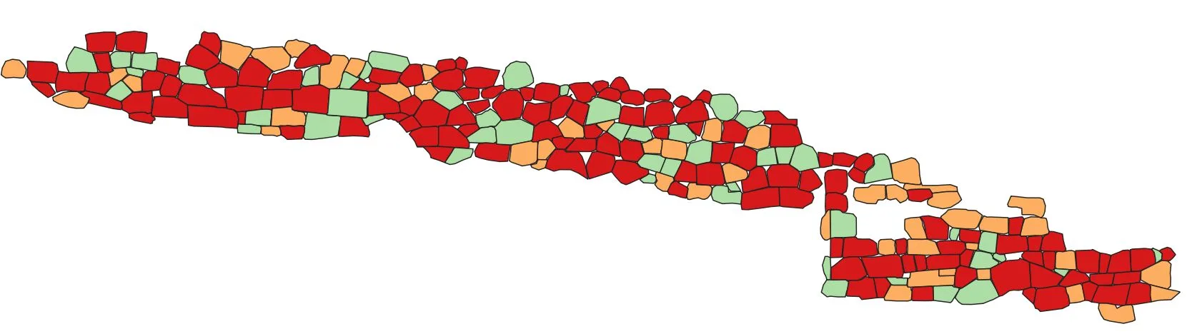
In this article we will explain how to automate the collection of statistical data on the metrology used in ancient masonry facings, using QGIS. Extracting quantitative data on ancient construction techniques in order to compile tables useful for metrological and/or mensiochronological assessments is a fairly lengthy task, requiring laborious data-acquisition work in the field. In the example presented in the following paragraphs, we have kept the field data-acquisition phase to a minimum, concentrating our efforts instead on making profitable use of the digital tools that can assist us in this analysis.

Background and starting data

For this article-tutorial we will use some data collected as part of the Archaeological Mission to Çuka e Ajtoit (Albania), specifically from the survey of the facade of Gate 1, built in the Hellenistic period in monumental polygonal masonry. The survey was carried out through photogrammetry, with images acquired using drones. This article will not cover the initial phases of the survey, i.e. image acquisition, image alignment, and the creation of the point cloud and final orthophoto. Instead, we will start from a finished product, namely the stone-by-stone survey carried out in a GIS environment, with a line layer drawn over the orthophoto.

The layer, in Geopackage format, can be downloaded from this link.

1. Data cleaning: converting polylines to polygons

The first step is to convert the polyline layer into polygons, so that each stone/element is represented by a polygon. This step can be skipped if your starting survey already uses polygons.

The first step therefore requires loading our example layer into a new QGIS project:

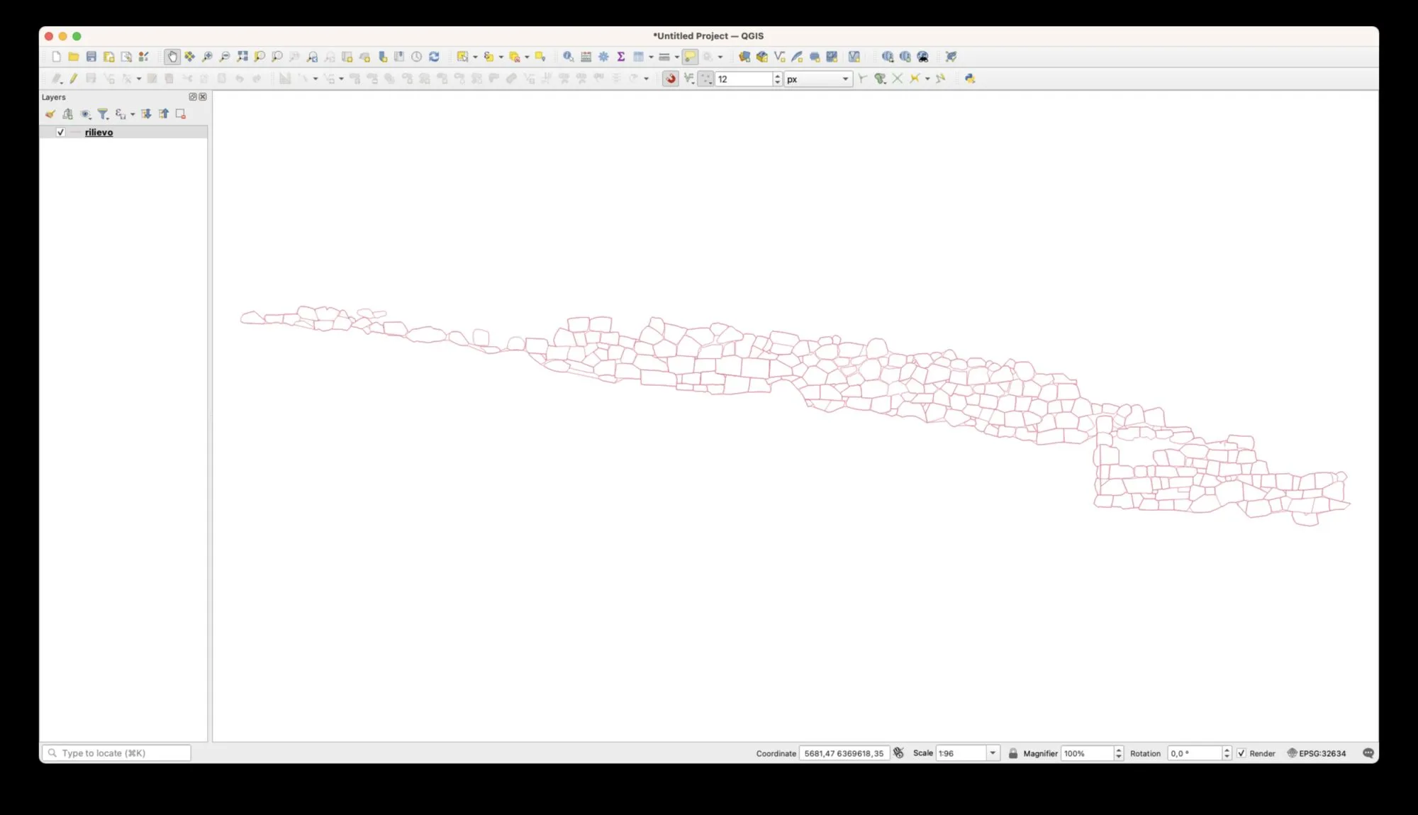
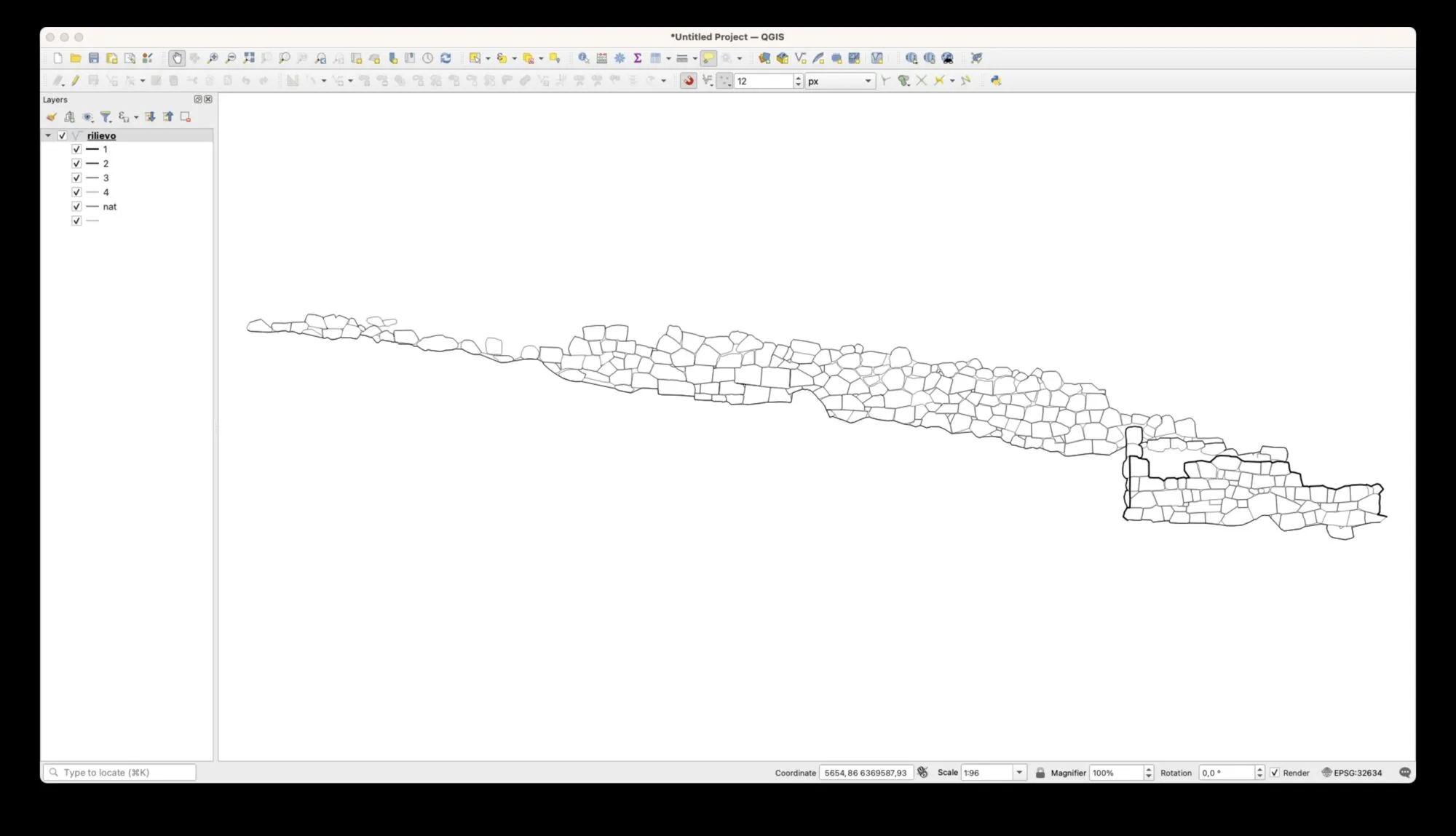
If you look at the attribute table, you will notice that this file uses the type field to encode some elements other than blocks, specifically the lines marking a difference in depth from the plane.

Applying a categorized symbology, we can obtain the following view:

For our analysis we only need the lines that define the blocks, so we can apply a filter to remove the others. For this we can use QGIS’s Query Builder tool:

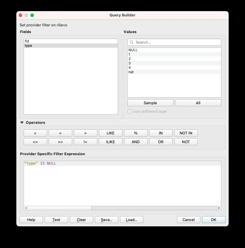
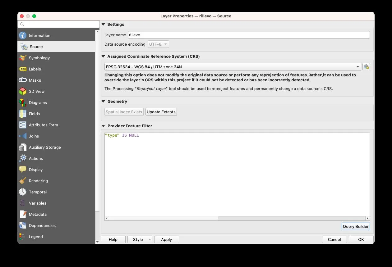
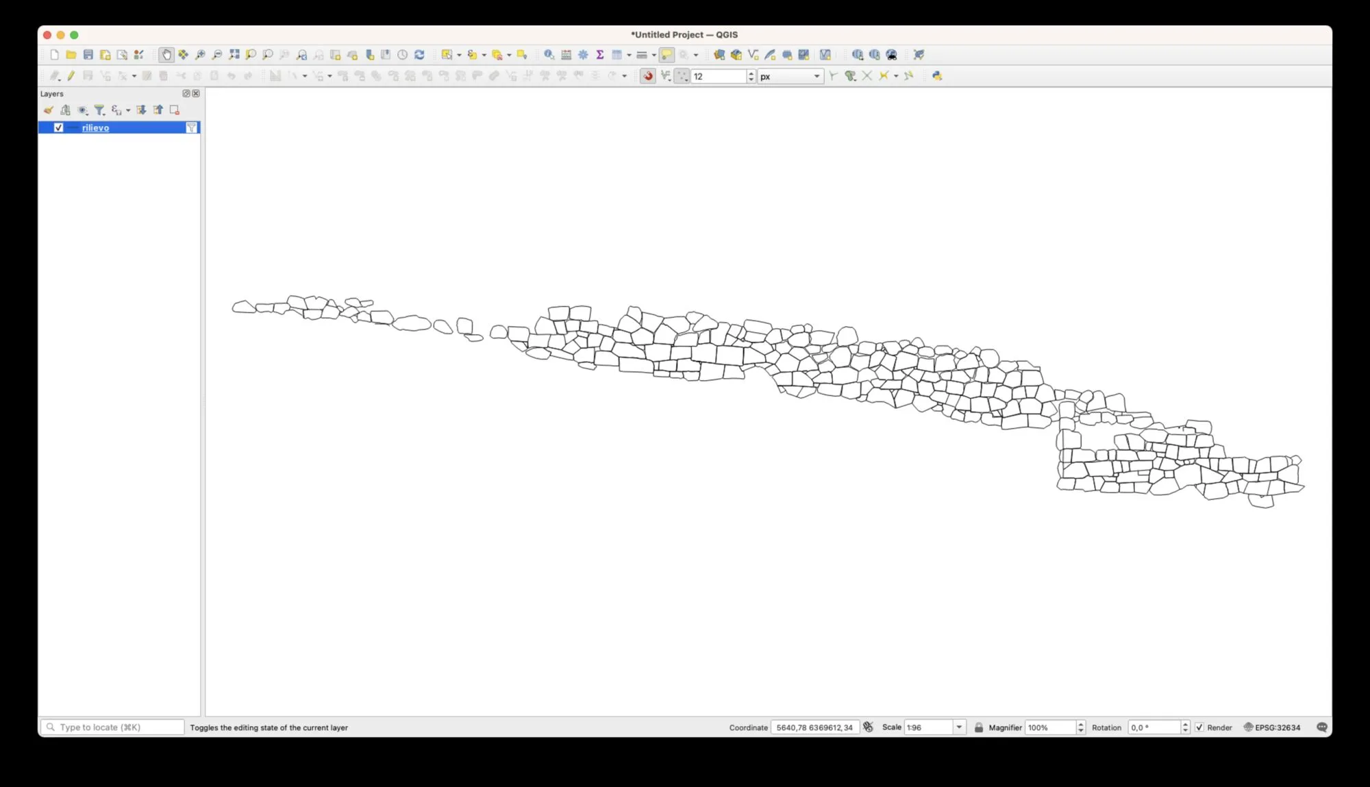
The expression "type" IS NULL allows us to filter and display only the elements that have a NULL value in the type field. We thus obtain a layer that shows only the geometries we are interested in:

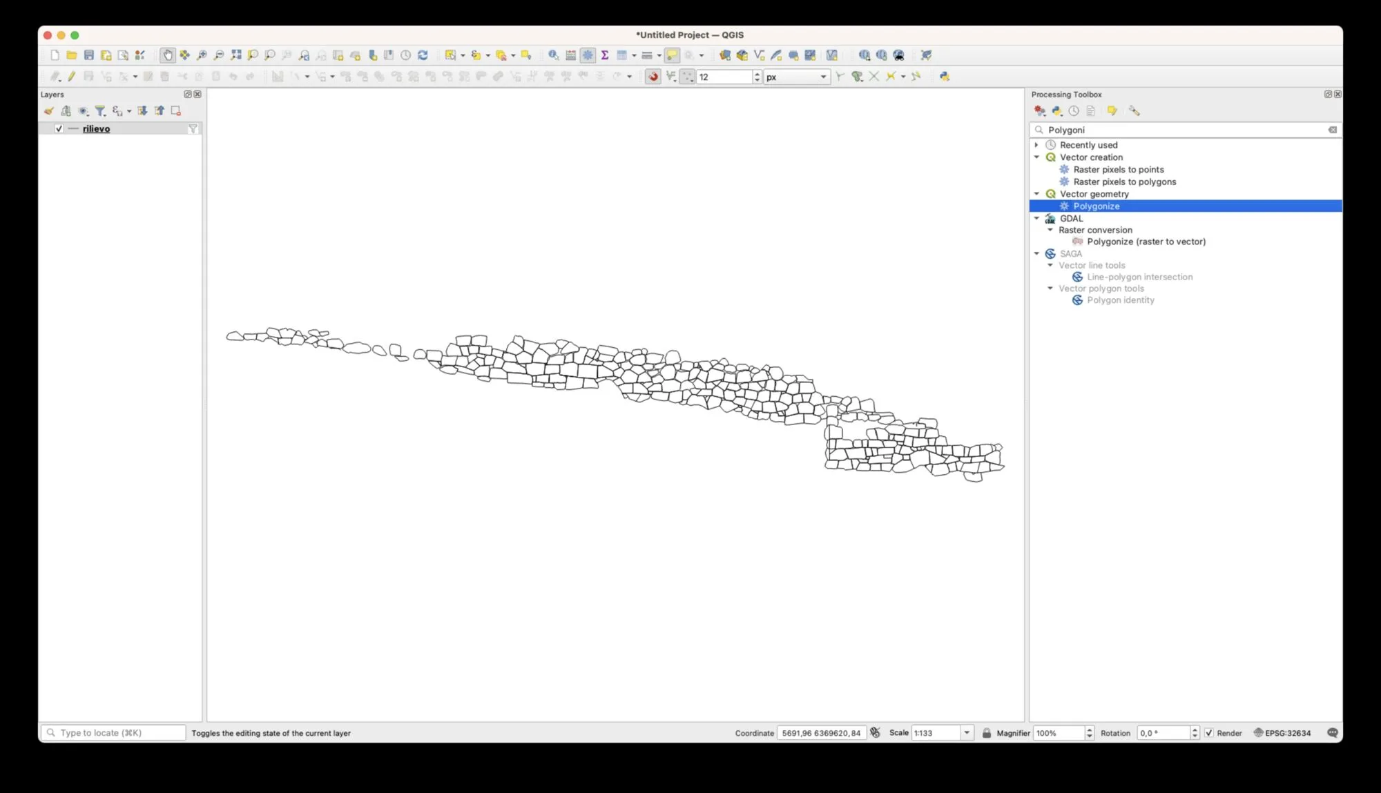
At this point we can use QGIS’s Polygonize tool, found in the Processing panel, accessible from Processing menu > Toolbox:

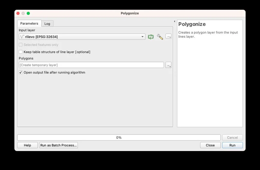
We can leave the default options in the tool’s window and use a temporary layer for the result of our analysis:

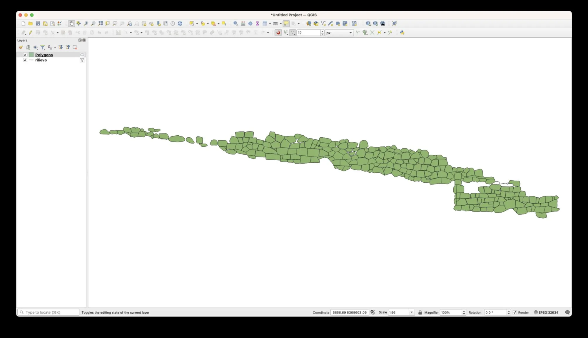
If everything went well, the Polygons layer should be added to the layers list, and we should be able to see a result similar to the image below:

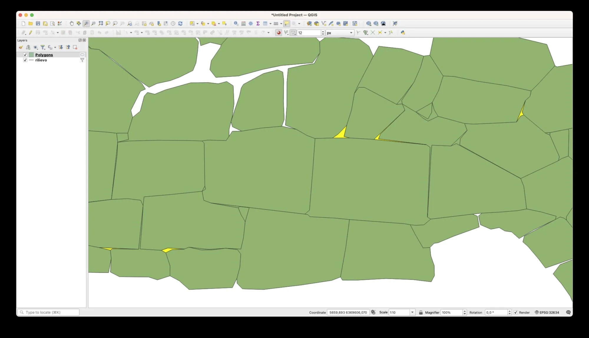
If we look closely at the result, we can notice that QGIS has also created some polygons that we do not need, such as the gaps between the blocks, highlighted in yellow in the following figure:

We could certainly delete them manually, but that would be a lengthy operation, so let’s try to automatically select all the polygons whose area is too small to be blocks. To do this we need to add an attribute containing the area of each polygon, which we can easily do with the Field Calculator tool:

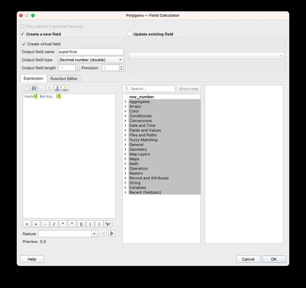
The expression entered, round( $area, 2), will return the area of each polygon, which for convenience we round to two decimal places using the round(n, 2) function. We call the new virtual field superficie and select Decimal number (real) as the field type.

We can check whether the operation was successful by opening the attribute table of the Polygons layer:

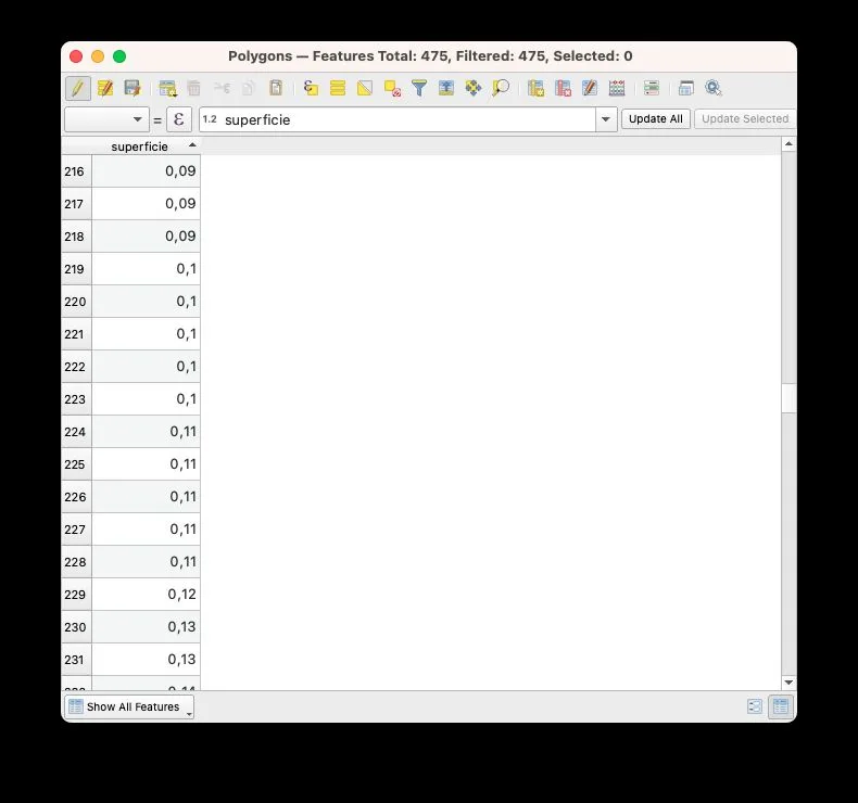
At this point we can select and then delete all the polygons that are too small, e.g. with an area smaller than 0.1. Let’s click on the Select Features Using an Expression icon

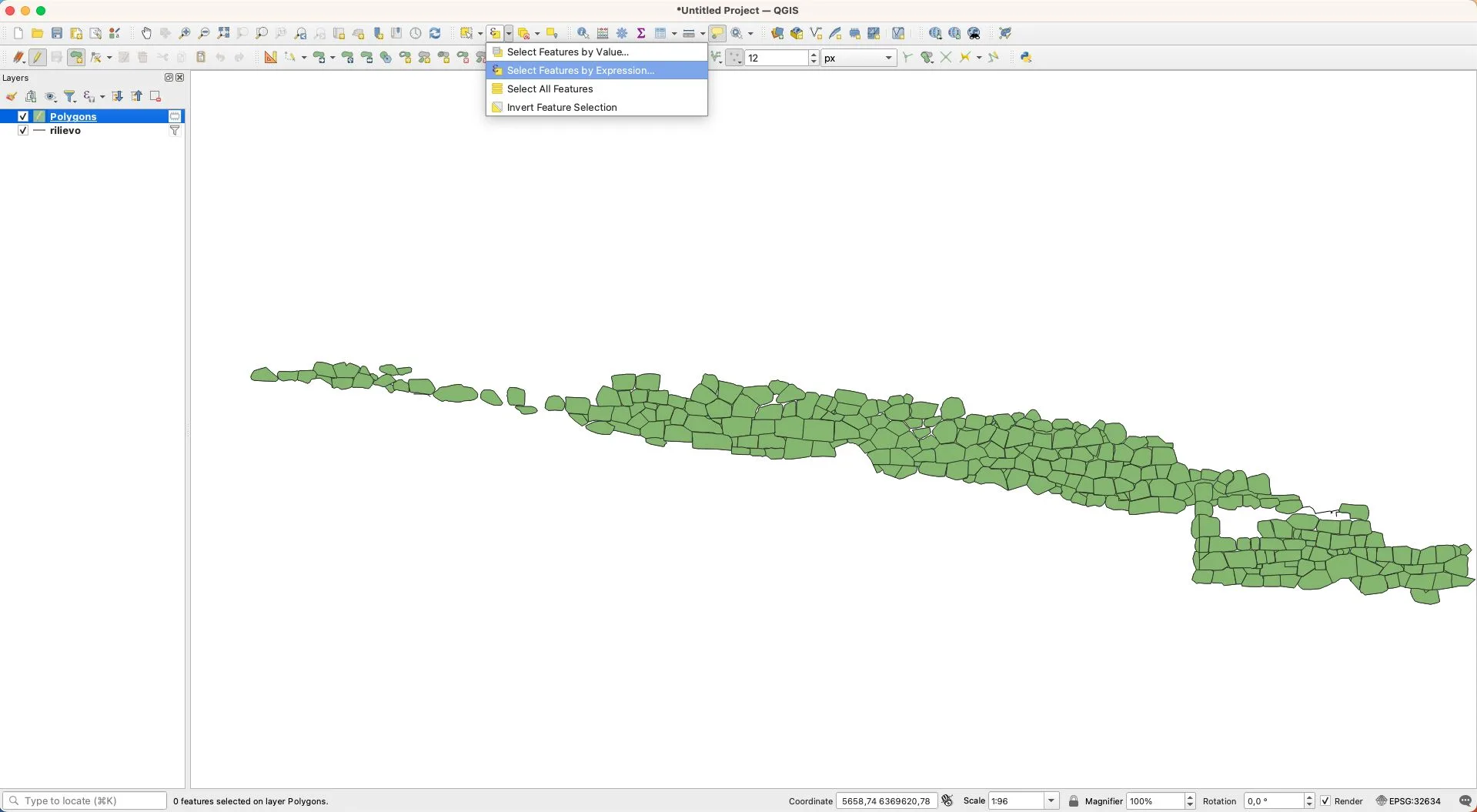
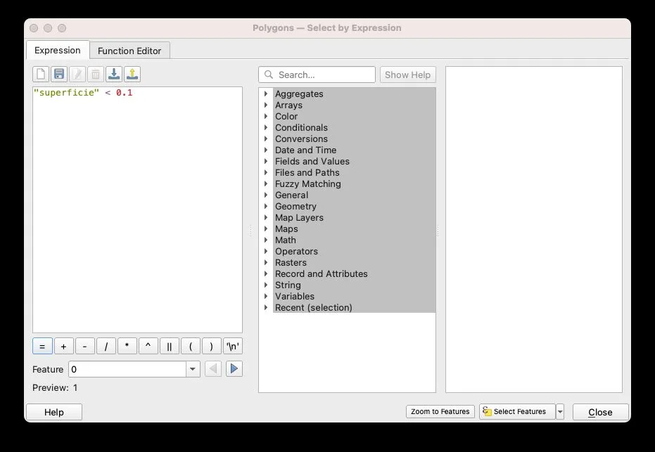
In the expression window, we write or paste the following expression, which allows us to select polygons with an area smaller than 0.1: "superficie" < 0.1, and then click Select features and then Close:

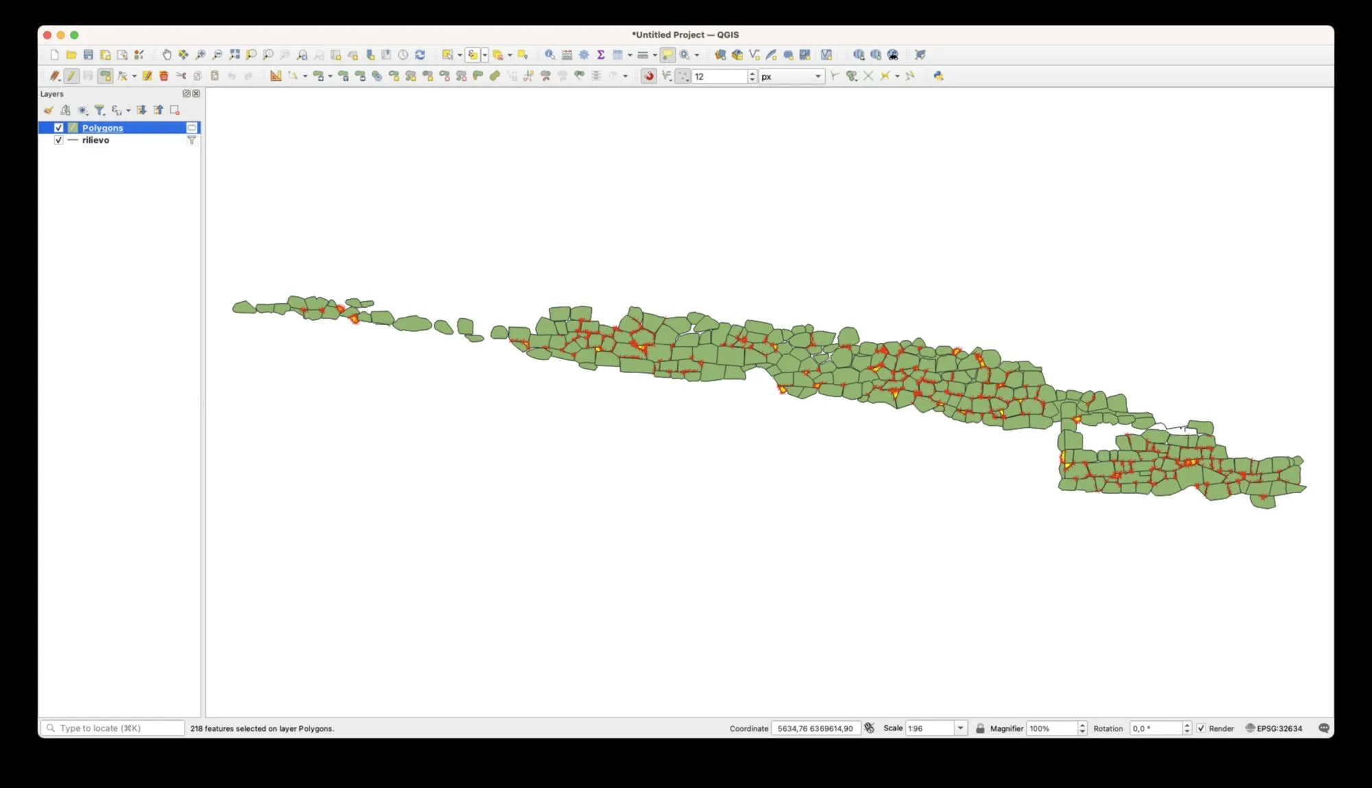
At this point we should have selected all the unwanted polygons, as well as a few smaller blocks which, for the current example, do not pose a statistical problem, since they are simply small filler stones (chinking) and can therefore be deleted.

Any remaining issues can be resolved manually.

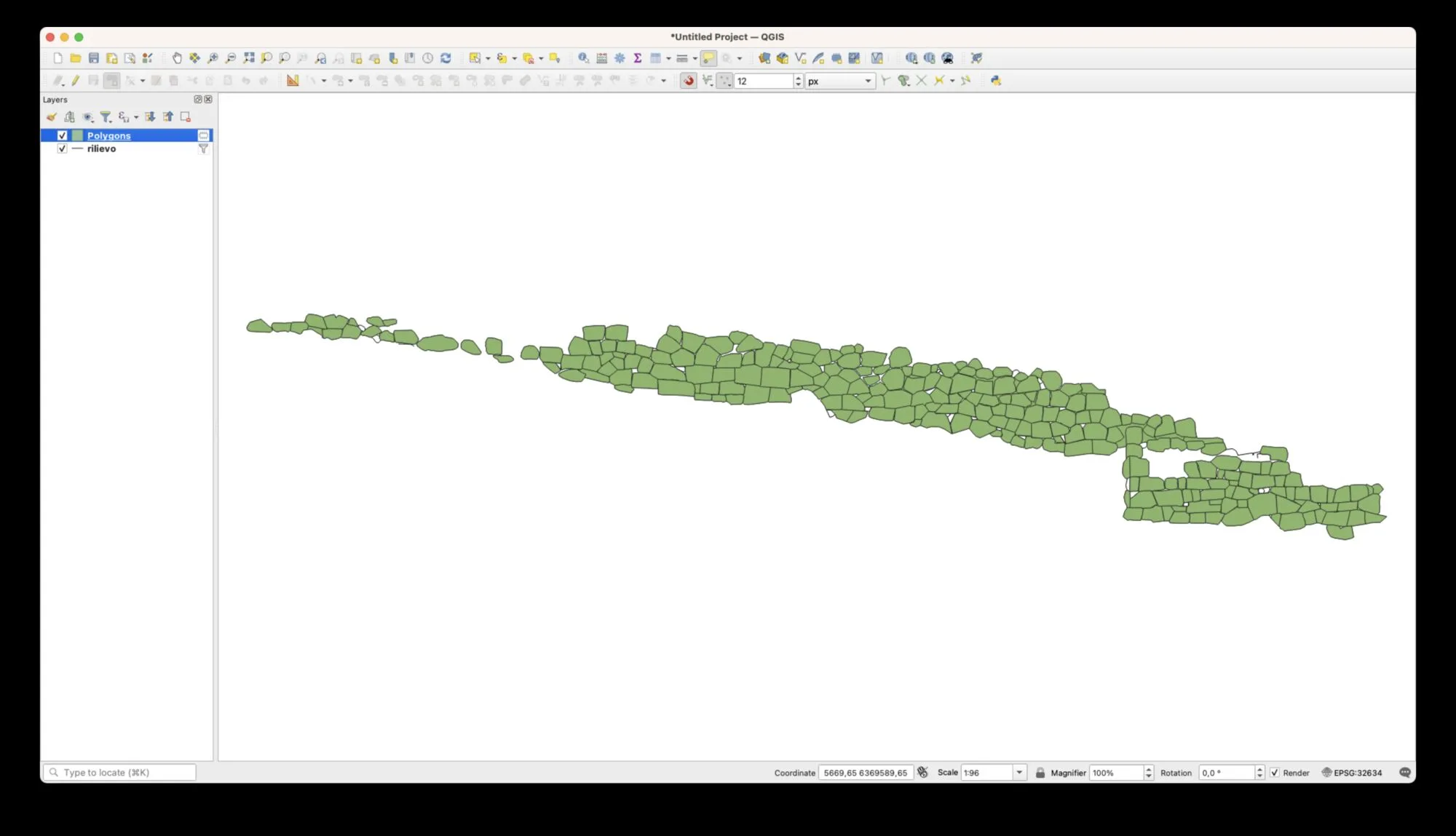
We can now finally delete the selected polygons and save the layer:

2. Creating minimum bounding rectangles for measurements

To calculate the dimensions of each block we have a specific QGIS tool called Oriented minimum bounding box, found in the usual Processing panel:

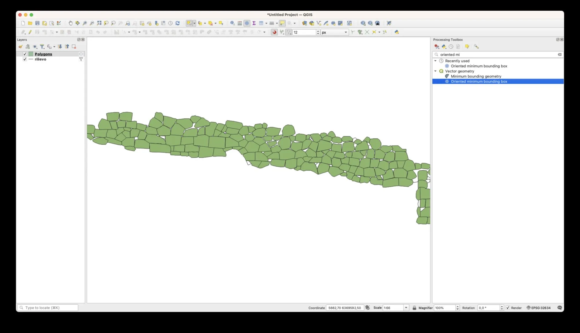
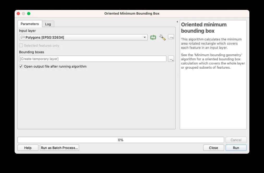
Once again the default settings are fine, and we create a temporary layer:

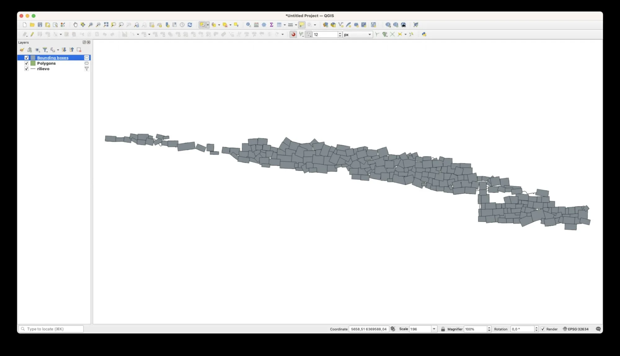
For each polygon in the layer, the algorithm creates a rectangle that perfectly circumscribes it, defining, as the name suggests, the minimum bounding rectangle. The graphic result is fairly confusing in our example, because the polygonal blocks have very different orientations from one another. The more regular the masonry, the more closely the resulting rectangles will match the underlying polygons.

What interests us most is the attribute table of the newly created layer:

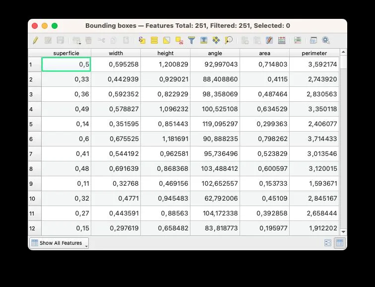
For each rectangle created, QGIS has in fact added the following attributes:

• width: the width
• height: the length
• angle: the orientation angle
• area: the area of the rectangle (always greater than the value reported in superficie)
• perimeter: the perimeter of the rectangle

Of these, the attributes that interest us most are width and height, which represent the larger dimensions of our blocks.

At this point we have all the data needed for our analysis, and we could extract it and process it with other statistical software, but we can also continue the analysis in QGIS.

3. Transferring the attributes to the survey polygons.

Since the bounding rectangles are not particularly meaningful in terms of their geometry, we can transfer their attributes to the original polygons. For greater precision in this operation, we will do so by creating centroids for each rectangle. Let’s select the Centroids algorithm from the processing panel:

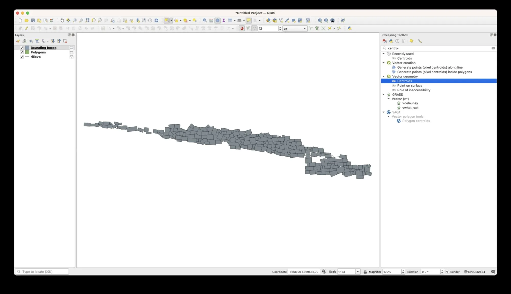
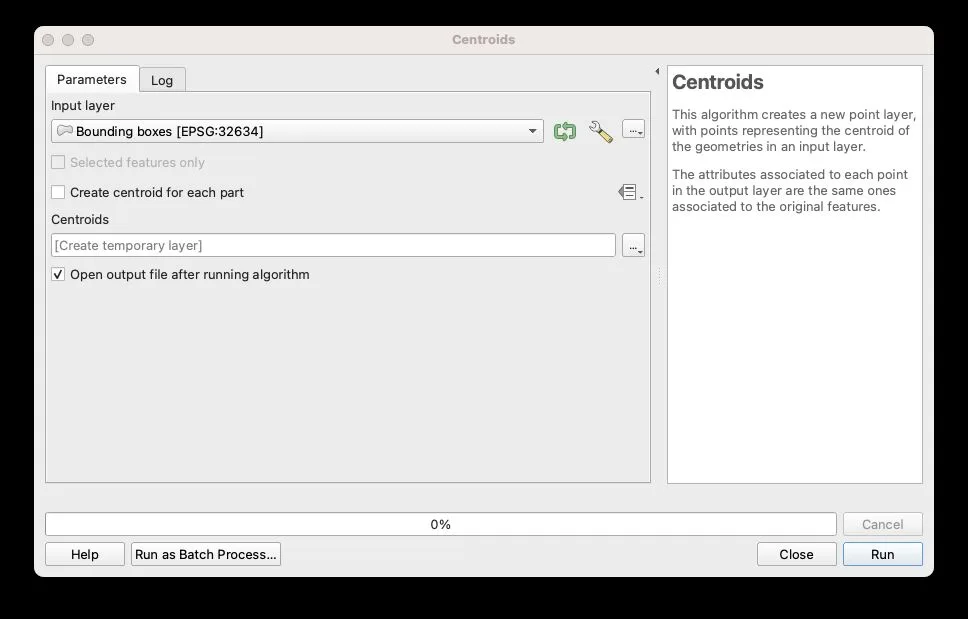
We use the default settings and create a temporary layer:

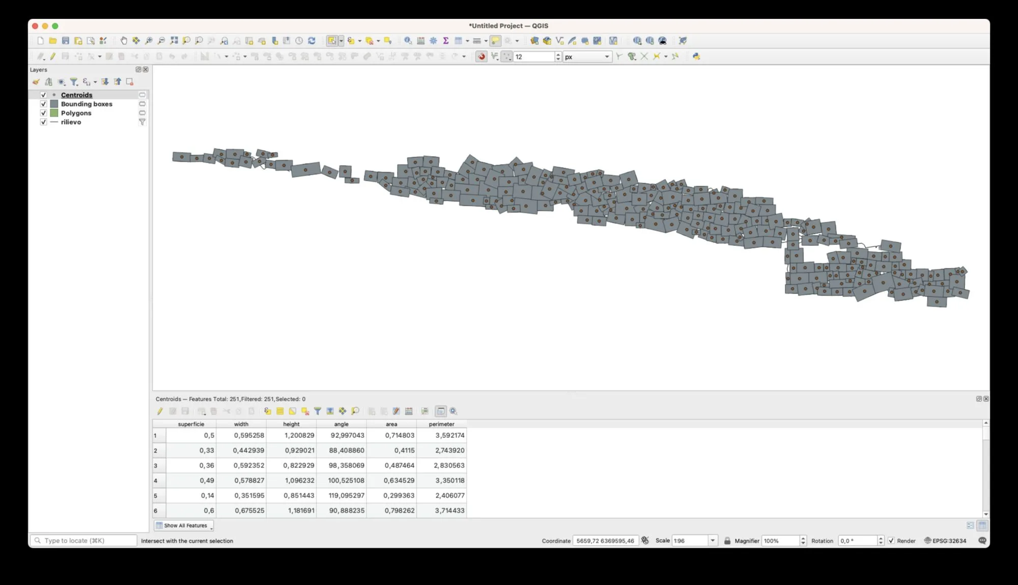
If everything went well we should obtain a point layer, representing the centroids of each rectangle, together with their attributes:

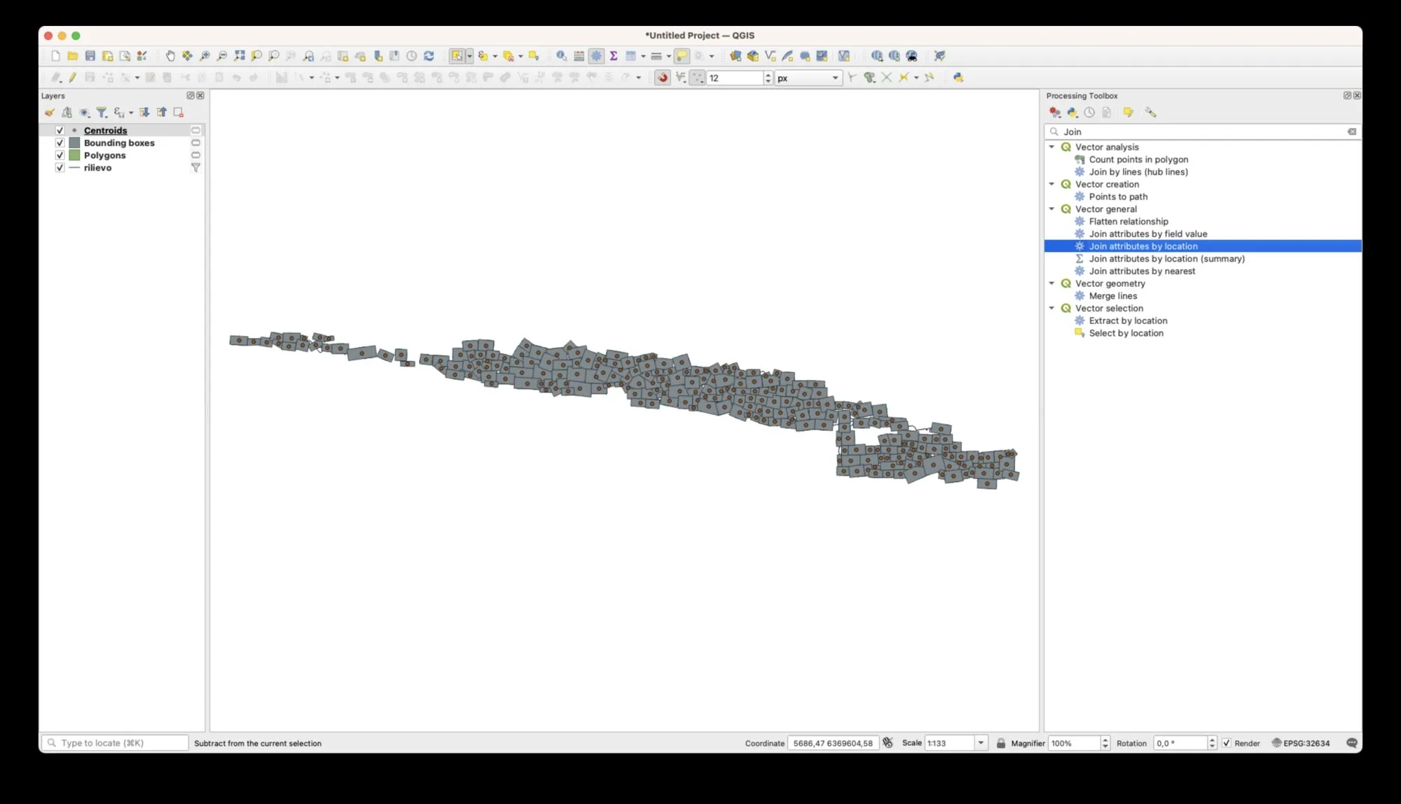
At this point we can use a spatial join to merge the attributes of Centroids with the geometries of Polygons. Let’s select the Join attributes by location algorithm from the Processing panel:

In the options window, we select Polygons as the Base layer — i.e. the layer whose geometries are to be used — and Centroids as the Join layer, i.e. the layer from which to take the attributes.

Select contains as the geometric predicate to use for the join, and leave Fields to add empty so as to import all the fields (optionally you can also select only width and height, which are the only ones useful to us).

As the Join type, select Create separate feature for each matching feature (one to many), even though in our case there should not be more than one centroid per polygon. This option will create two or more identical geometries in case there are multiple points within a single polygon. In that case, the duplicates will need to be resolved manually.

Finally, we leave the default option of creating a temporary layer for the results.

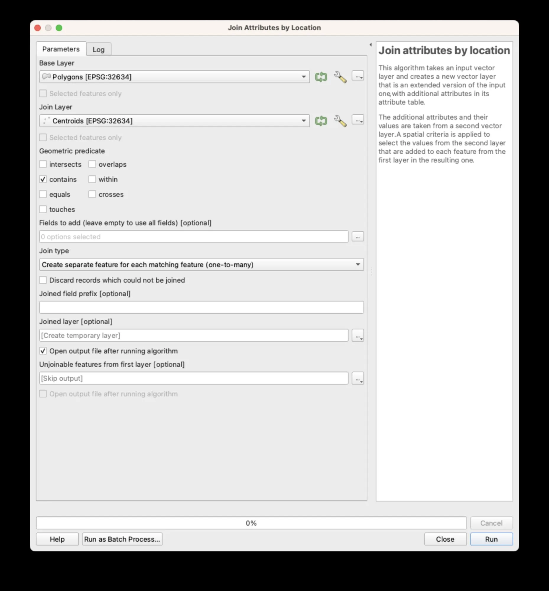
If everything went well we should obtain a result like the one in the image below:

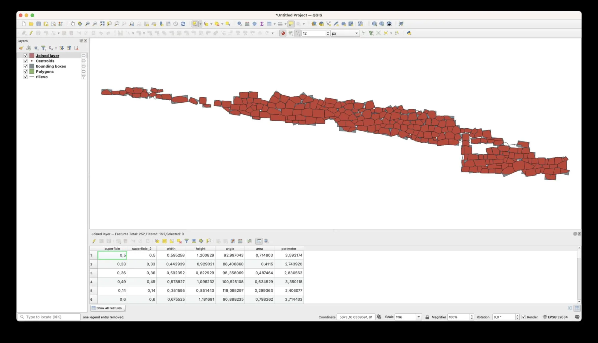
As can be seen in the attribute table, the superficie field is duplicated, but this field is not very important to us. In the next steps we will see how to clean up the data

Cleaning up the final layer and converting the units

At this point we can permanently save our layer and do a bit of cleaning up before the visualization analysis.

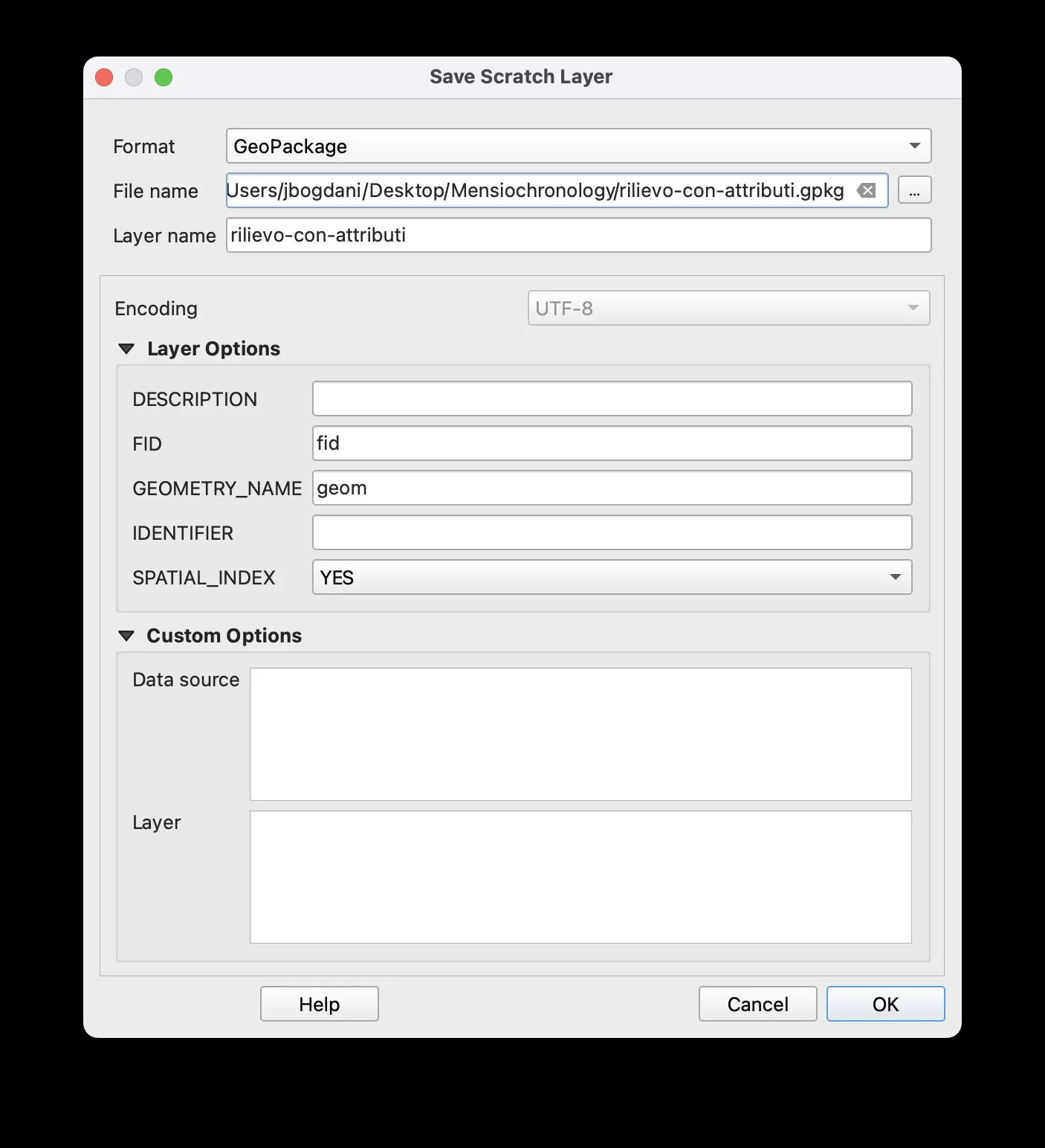
Let’s click on the small icon to the right of the layer’s name in the Layers panel (the “Make Permanent” action) to save the data to disk, and choose the GeoPackage format with the name rilievo-con-attributi.

Right-click on the layer in the Layers panel and select Properties. In the window that opens, go to Fields and delete the attributes we don’t need, namely: superficie, superficie_2, angle, area and perimeter.

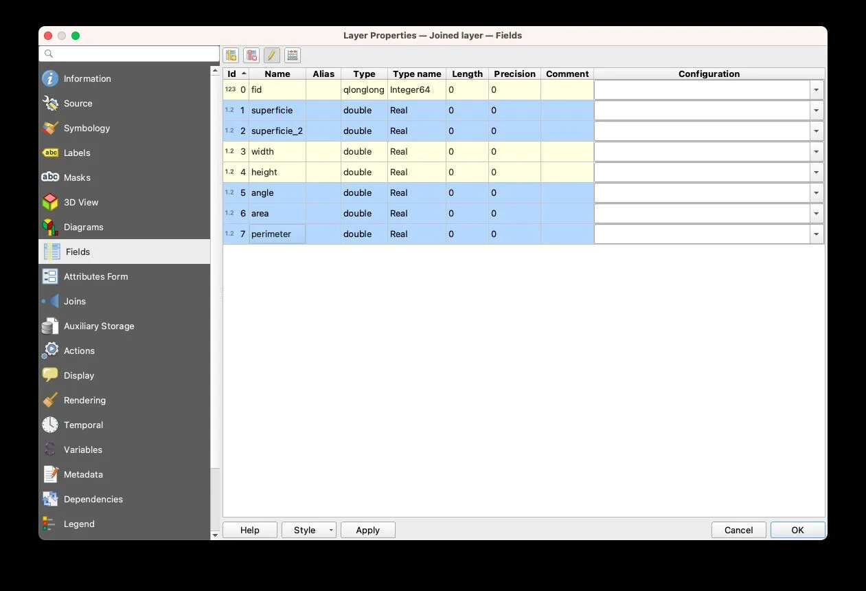
We should obtain:

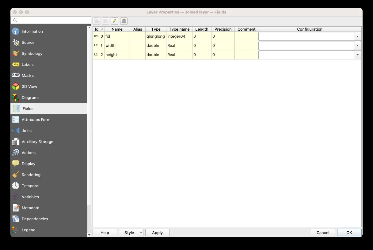
We are now ready to convert our measurements from metres into ancient units and to check whether that unit was actually being used. The ancient units in the Greek (and Roman) world are the foot and the cubit (1.5 feet), but the absolute length of the foot varies across space and time. For this reason, we will not use a fixed value for the foot, but will instead run several tests, using different absolute measurements.

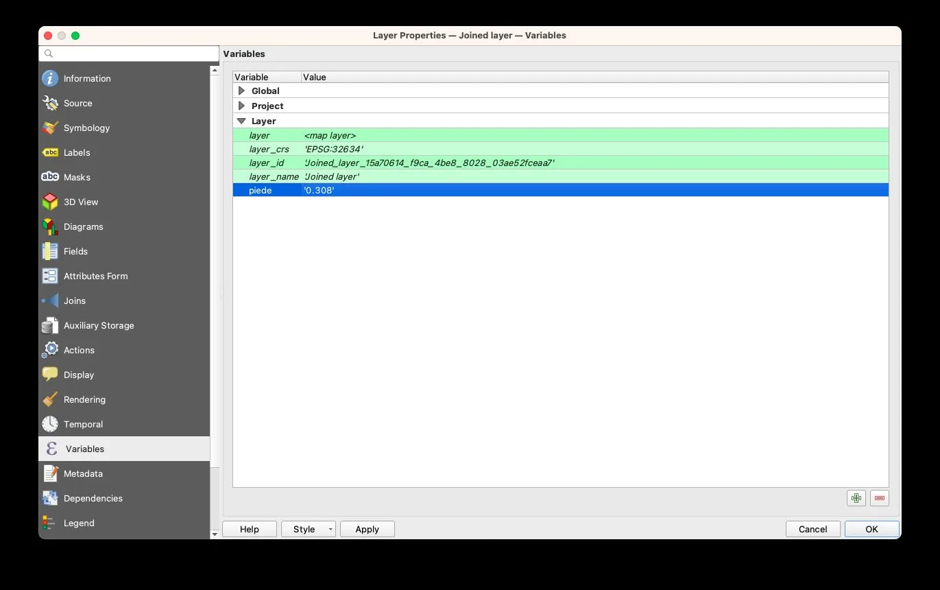
For this reason, we will define a variable within the layer that we can change at will, automatically obtaining updated calculations.

In the same properties window, we go to Variables and define a variable called piede with the value 0.296, which is the canonical measurement of the so-called Attic foot:

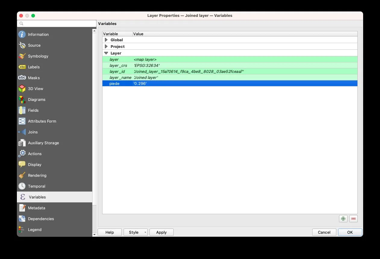
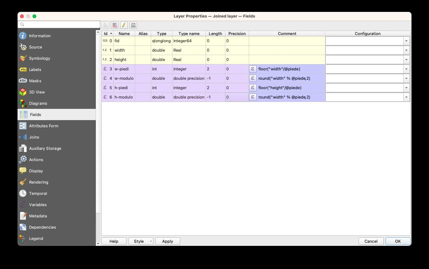
Let’s click Apply at the bottom, go back to Fields, and start our calculations, adding four virtual fields which will respectively contain:

• w-piedi: the conversion of the width measurement into feet, rounded down
• w-modulo: the modulo of the conversion of the width measurement into feet, i.e. the remainder of the division. This value measures the deviation from the ideal unit in the construction of the structure.
• h-piedi: the conversion of the height measurement into feet, rounded down
• h-modulo: the modulo of the conversion of the height measurement into feet, i.e. the remainder of the division. This value measures the deviation from the base unit in the construction of the structure.

Let’s click on the Field Calculator icon and start entering the data for the first field, as shown in the image:

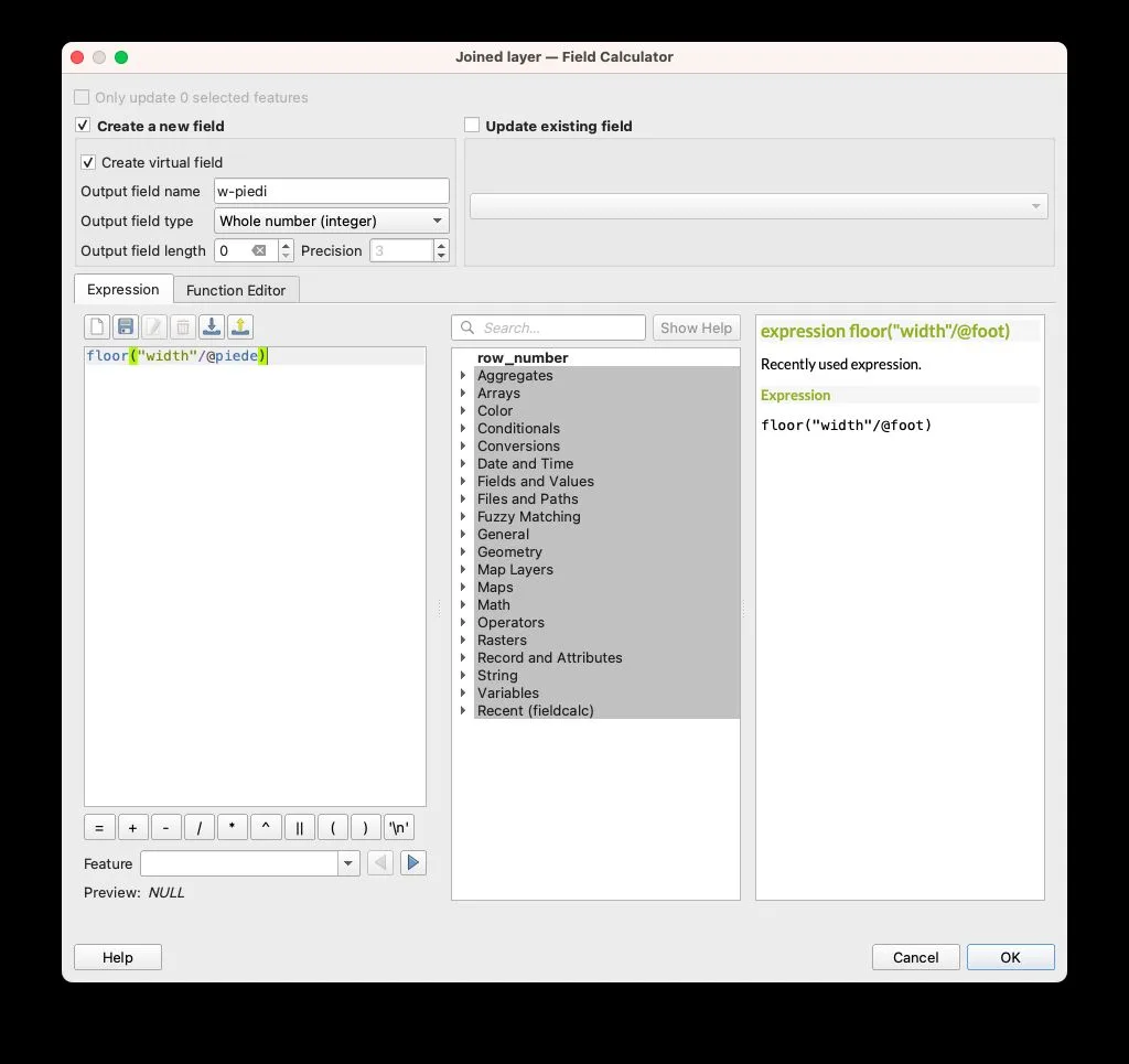
The expression floor("width"/@piede) is fairly straightforward: we are dividing the width measurement by the piede variable and rounding the result down to the nearest whole number.

Important: remember to:

• select the Create virtual field option, so that the data can be automatically updated whenever we update the piede variable
• select Whole number as the Output field type
• enter 2 as the Output field length

Let’s repeat the operation for w-modulo:

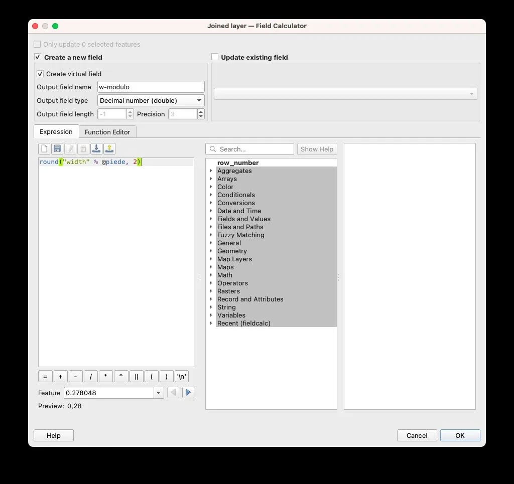
In this case we select Decimal number (double) for Output field type, since we expect a remainder in centimetres, always smaller than the length of the foot.

The expression round("width" % @piede, 2) rounds to two decimal places (round(n, 2)) the result of the modulo (%) calculation of the width measurement with the piede variable.

Let’s repeat the two operations above for the height field as well, changing w to h and width to height where necessary, to obtain:

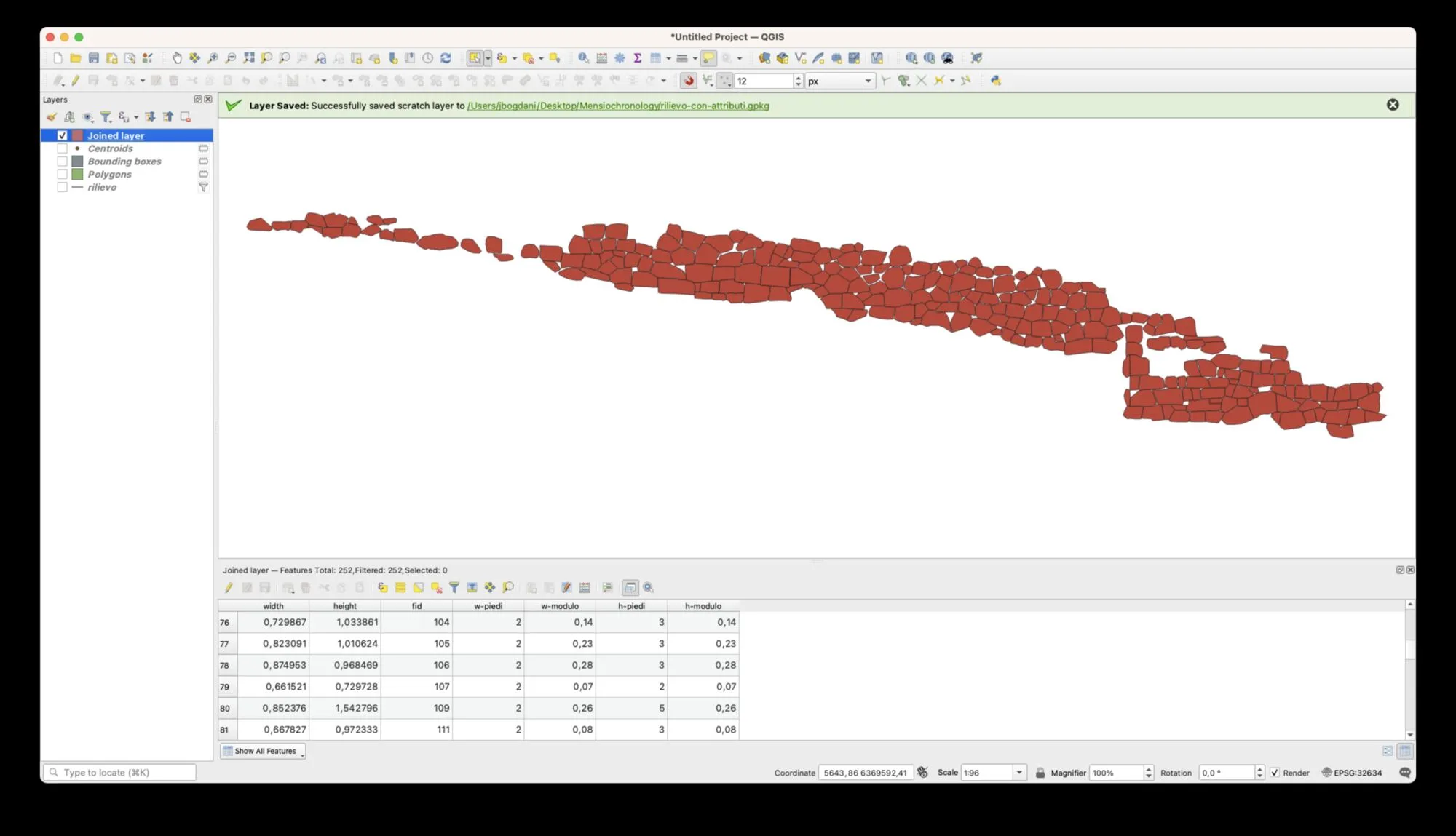
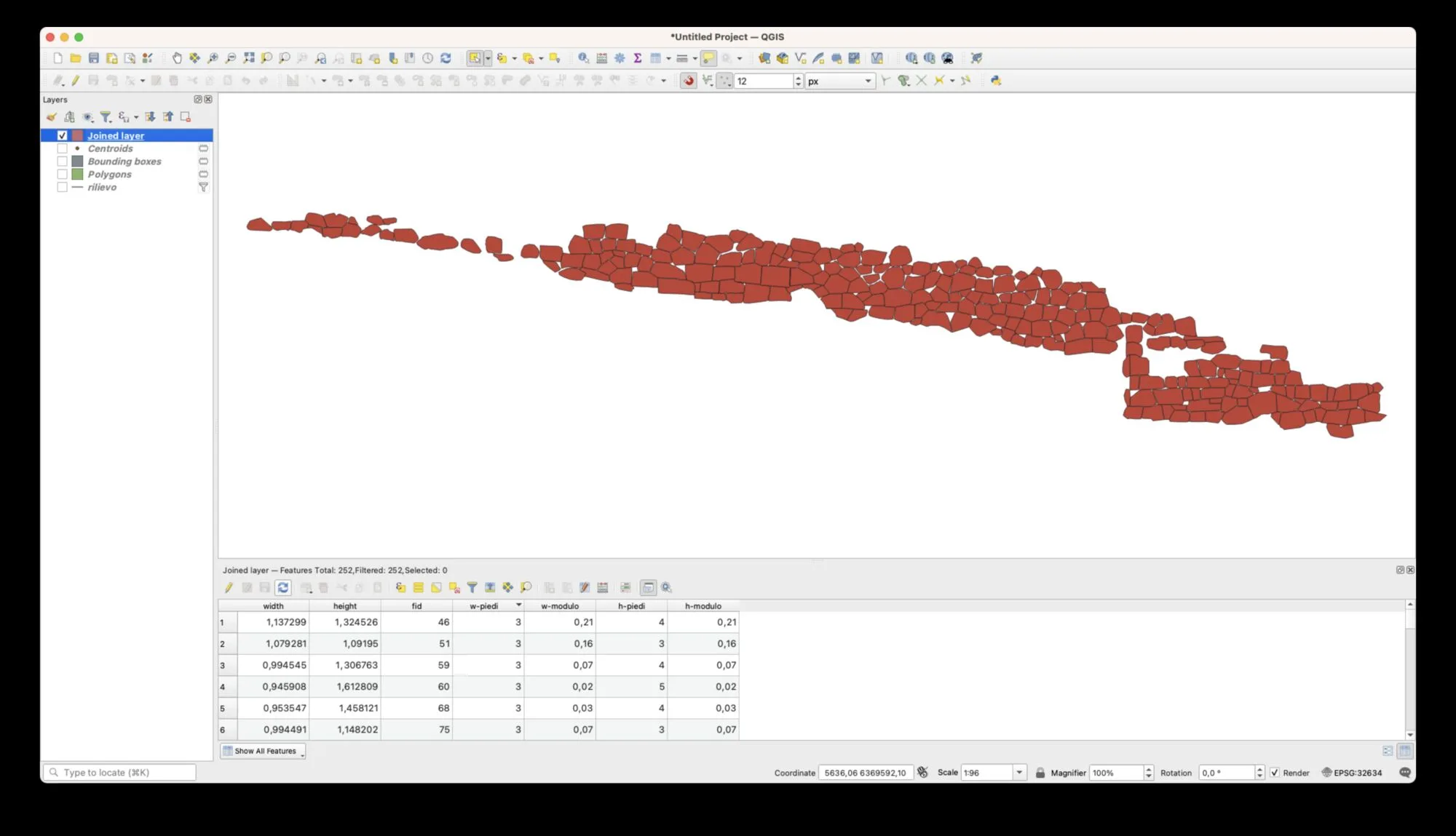
At this point we have all the data we need. This data is dynamic and depends on the piede variable. If, for example, instead of the Attic foot we want to use the Olympic foot of 30.8 cm, all we need to do is update the variable, and the values of the w-piedi, w-modulo, h-piedi and h-modulo fields will be updated automatically:

4. Visualizing the data

At this point, we can use different colours to visualize how far each block deviates from a round measurement (and multiples) of the foot. Everyone can decide on different visualization criteria, but for simplicity we will define three distinct classes:

• Good adherence to the standard: this includes all the deviation (modulo) values of width (i.e. w-modulo) from 0 (perfect adherence to the foot) up to a tolerance of +3 cm. This class will also include the high values of w-modulo (measurements approaching the next foot), again with a tolerance of 3 cm;
• Average adherence to the standard: this includes w-modulo values that deviate from 3 to 6 cm from the round measurement (0 at the low end, or close to the value of the foot at the high end);
• Poor adherence to the standard: this includes the remaining measurements, i.e. those that deviate by more than 6 cm from the measurement chosen as the standard (the piede variable).

We can turn the 3cm measurement into a parameter, as a variable, so that it can easily be changed centrally.

Below is a step-by-step guide with annotated images:

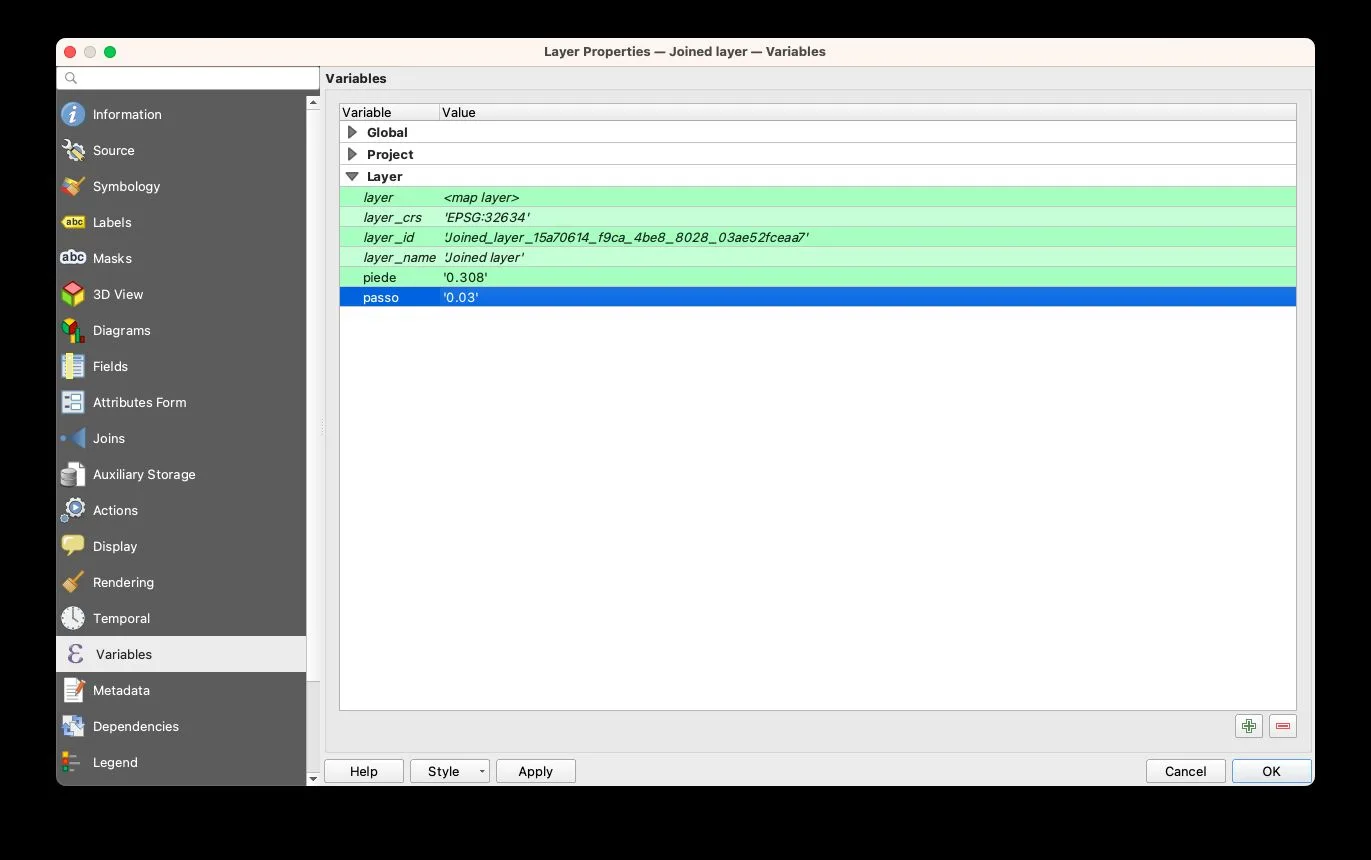
I configure the passo variable with the value 3cm.

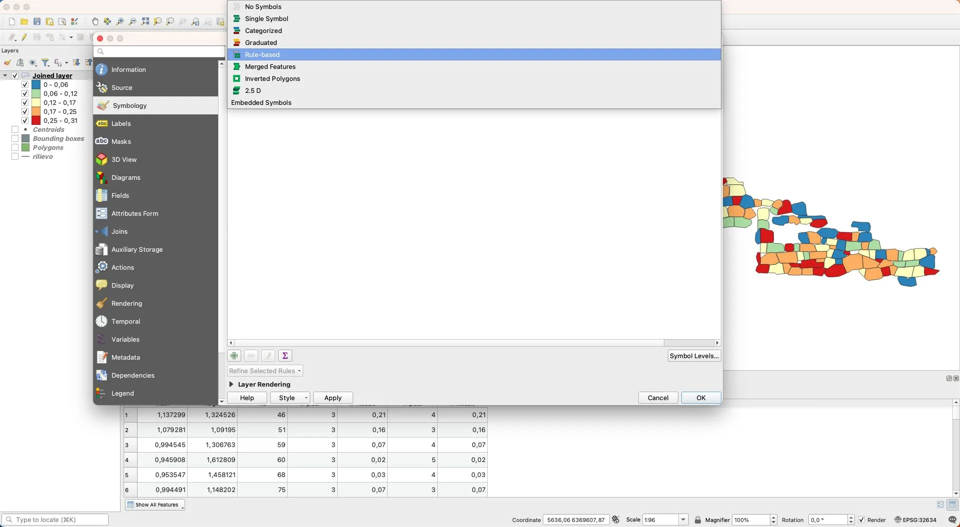
In Symbology we select Rule-based and define our three classes:

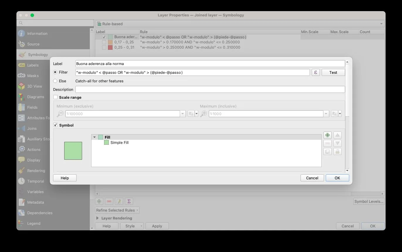
The Good adherence to the standard class is defined by the expression: "w-modulo" < @passo OR "w-modulo" > (@piede-@passo), i.e. all w-modulo values less than the passo variable (currently 3 cm), and all w-modulo values greater than the value obtained by subtracting the passo variable (3 cm) from the piede variable (29.6 cm), i.e. 26.6 cm.

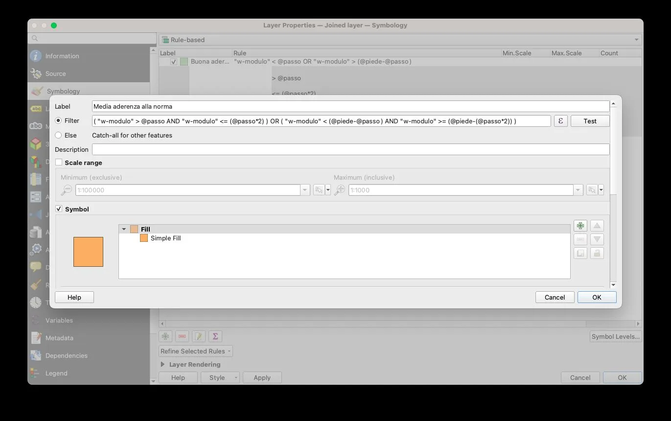
The Average adherence to the standard class is defined by the expression:

1
(
2
  "w-modulo" > @passo
3
  AND
4
  "w-modulo" <= (@passo*2)
5
)
6
OR
7
(
8
  "w-modulo" < (@piede-@passo)
9
  AND
10
  "w-modulo" >= (@piede-(@passo*2))
11
)

These are all w-modulo values greater than the passo variable (currently 3 cm) and less than or equal to twice passo (currently 6 cm), together with all w-modulo values greater than or equal to the difference between piede and passo, and greater than or equal to the difference between piede and twice passo, i.e. greater than or equal to 29.6 − (3 × 2) = 23.6 cm.

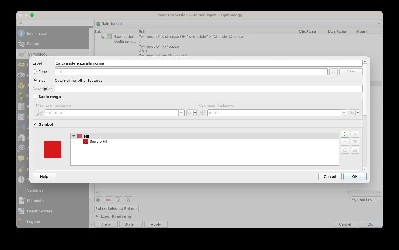
For the Poor adherence to the standard class, for convenience we can use the ELSE function, which groups together all the values not currently covered by the definitions given so far.

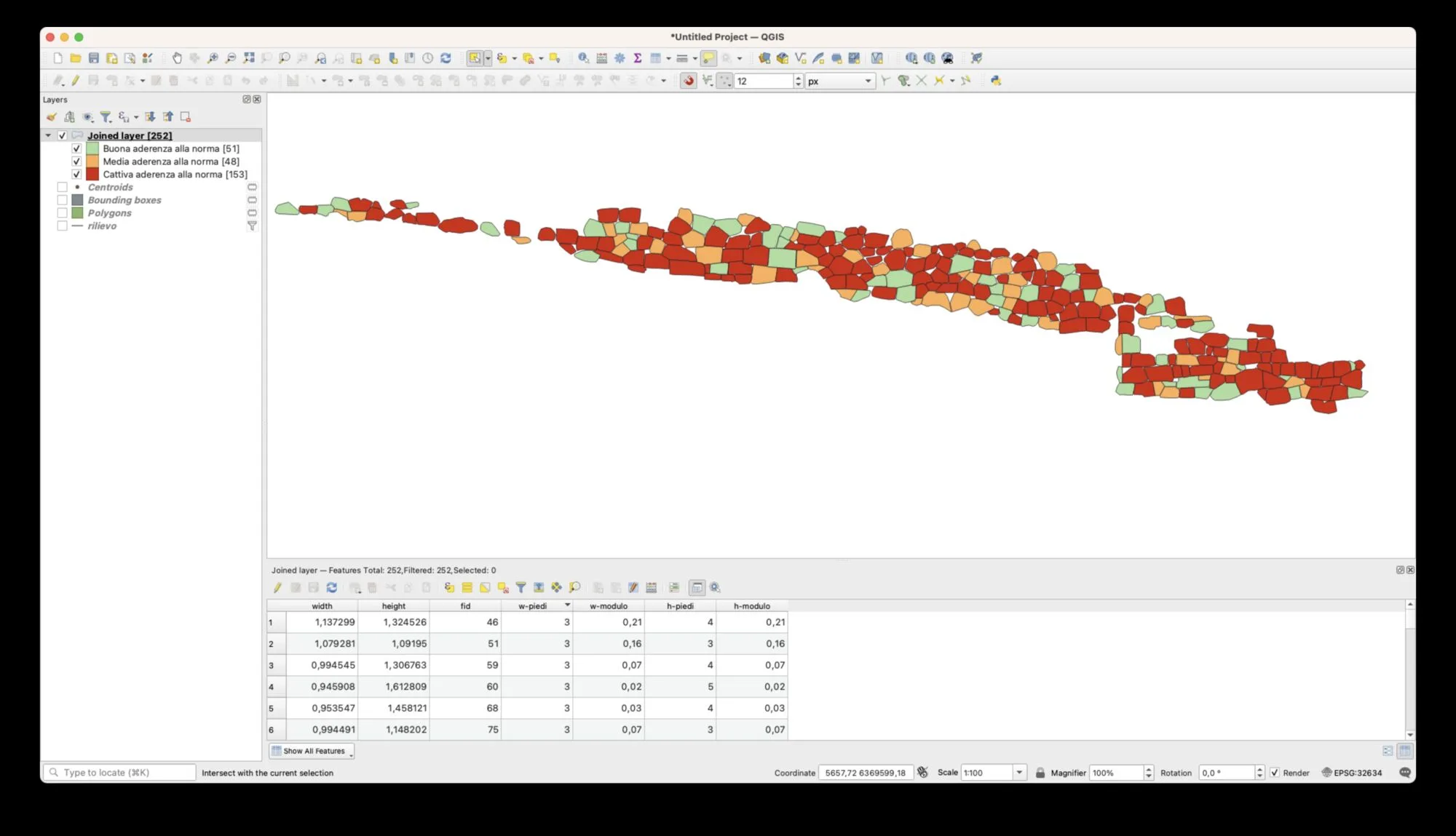
The image above shows the result of our analysis, using the Attic foot of 29.6 cm.

By changing the value of the piede variable to 0.308, i.e. the Olympic foot, the graphic results will update accordingly:

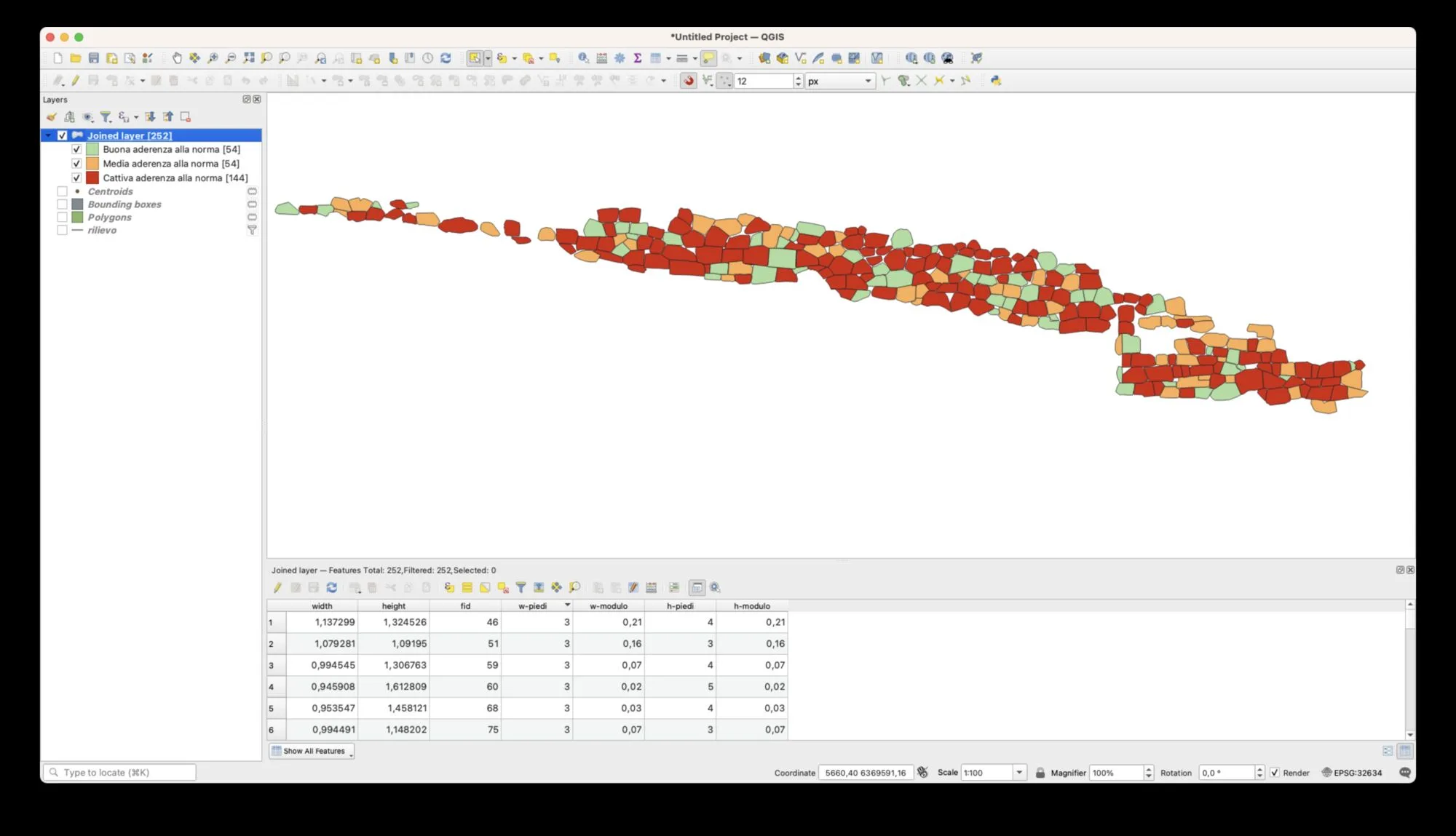
Naturally, we can also change the value of the foot to coincide with the cubit, or we can include in our symbology, within the Good adherence to the standard class, values close to the reference cubit (@piede * 1.5).

References

• Calculating the minimum bounding boxes of a polygon layer: https://gis.stackexchange.com/a/265233