

Introduction
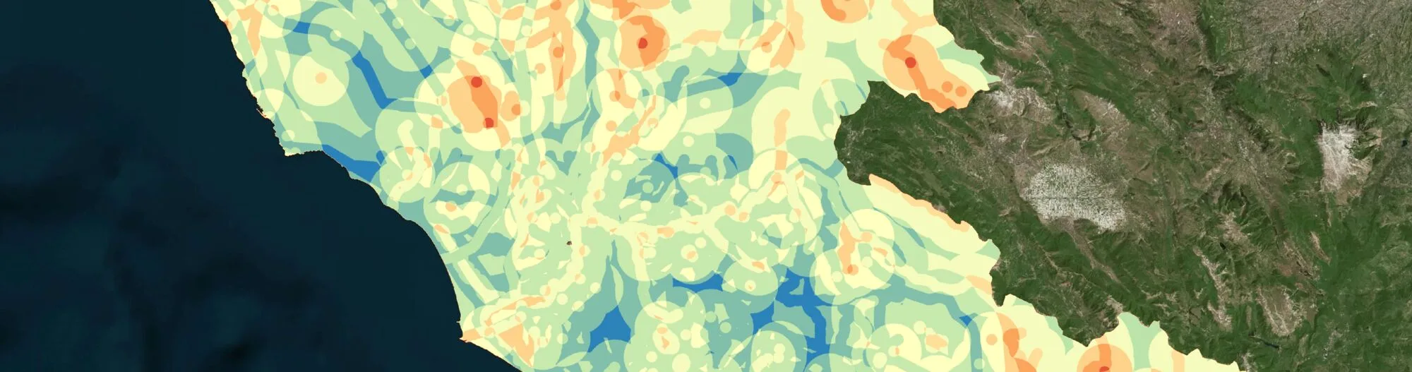
Every year LAD organizes GIS workshops open to Sapienza students and beyond. In the latest edition (academic year 2021/2022), during the Advanced GIS workshop we decided to adapt an example of multi-criteria weighted-overlay analysis, originally carried out on contemporary data, to a purely archaeological case. The experiment was very well received by all participants, and we therefore decided to publish it on our blog in the hope that it may be of help and inspiration to everyone working in the field of territorial analysis.
Multi-criteria weighted-overlay analysis is a process for classifying areas based on a set of attributes they are expected to possess, according to specific criteria chosen by the user.
In this guide we will look at a use case of multi criteria weighted-overlay analysis using QGIS software. We will consider a concrete case study, an archaeological question relating to a well-defined chronological and geographical context.
The archaeological question formulated is as follows:
Which areas of the present-day Lazio region present optimal characteristics for the development of Roman imperial-period settlements, but which, to date, have not yielded reliable traces in this sense?
In order to answer this concretely, to find the data needed for this type of analysis, and also to understand in practical terms which analyses will need to be carried out, it is necessary to spell out the request more clearly.
Non-archaeological guide available at: http://www.qgistutorials.com/it/docs/3/multi_criteria_overlay.html
A repository has been created providing access to all the data needed to follow the guide step by step: https://github.com/lab-archeologia-digitale/mcwoa-archeo/
The data
Geographic boundary
The geographic boundary is the simplest piece of information to understand and also the easiest data to find. The Lazio Region has well-defined administrative boundaries that are easily found online in GIS format; specifically, for this exercise the data was downloaded from: https://www.diva-gis.org/gdata
Optimal settlement characteristics: requirements, data, parameters
This is a much more difficult element to define and evaluate, and certainly much more subjective.
For the purposes of this exercise, only a few elements will be considered, with parameters decided a priori, though these can certainly be debated. Specifically, the following elements are considered particularly interesting, as they give a good sense of the attracting/repelling character of a given theme:
- proximity to the road network
- not too close to the water network, which has always been a source of risk, but not too far away either, since water is a “costly” resource to transport
- not excessive proximity to existing settlements, which “use up” the potential of an area
To calculate these variables we therefore need:
- a Roman imperial-period road network: compiled by the Ancient World Mapping Center and freely available in GIS format, at http://awmc.unc.edu/awmc/map_data/shapefiles/ba_roads/
- Inland water bodies (lakes) are likewise available courtesy of the Ancient World Mapping Center, in GIS format, at: http://awmc.unc.edu/awmc/map_data/shapefiles/physical_data/inlandwater/
- The river network was downloaded from https://www.diva-gis.org/gdata. This data does not refer specifically to the Roman period, so further work on it would be needed to make this analysis more accurate.
- The network of known Roman imperial-period settlements was instead downloaded from Pleiades, at: http://atlantides.org/downloads/pleiades/kml/pleiades-latest.kmz
- Finally, the digital terrain model (DEM) at 30m resolution was downloaded from https://opentopography.org/, through the
QGIS OpenTopography DEM Downloaderplugin
To make this guide easier to follow, we have downloaded and collected all this data in a single repository, which you can find at: https://github.com/lab-archeologia-digitale/mcwoa-archeo.
Analysis procedure
1. Starting the program and preparing the data
- Open a new QGIS project and load all the data present in the archive
- Group the vector layers (
fiumi-lazio,strade-lazio,acque-interne-lazioandinsediamenti-imperiali) into a group calledStep-1 - Save the project
2. Rasterizing the data
This exercise can be done either working with vector data or with raster data, obtaining different results. With raster data — the option chosen here — a more gradual result is obtained.
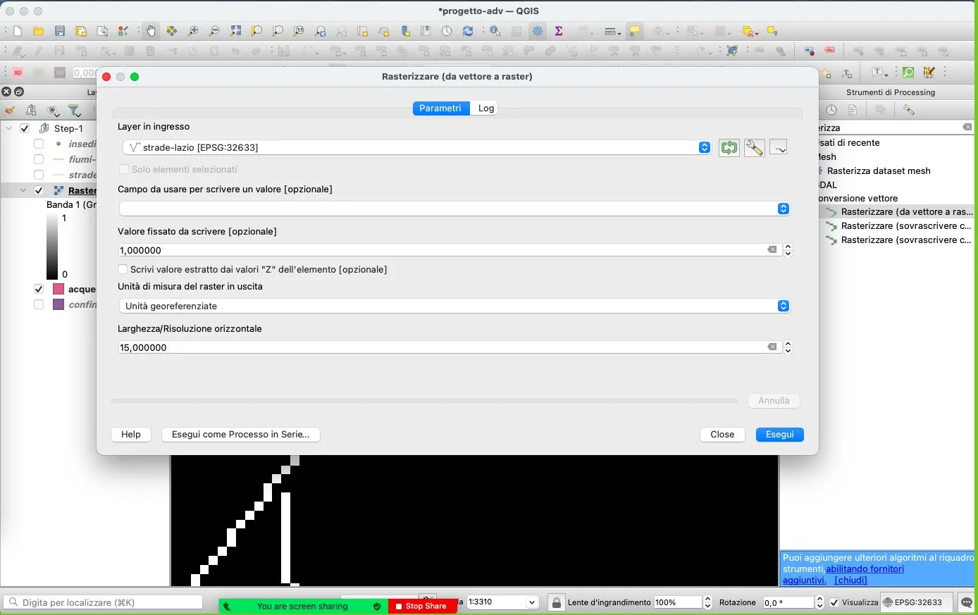
We then proceed to rasterize the vector data contained in the Step-1 group in QGIS, i.e. the process that produces raster data from a vector layer.
Processingmenu >Toolbox- In the panel that opens, search for and open the
Rasterize (vector to raster)tool - Under
Parameters, from the drop-down menu underInput layerselectstrade-lazio, the first layer to rasterize - Set the
Fixed value to burn [optional]field to1,000000.
With this setting, in the raster file the pixels corresponding to the extent of the vector will have the value1, the othersnull(see below). - From the drop-down menu of the
Output raster size unitsfield, selectGeoreferenced units.
This way, the units of the input data will be used — in this case metres, since the data is in an orthogonal projection. Care must therefore be taken here in the case of data expressed in geographic coordinates, where the base unit is the degree. - Set the
Width/Horizontal resolutionfield to15,000000.
This setting defines the width of the output pixel, i.e. 15 metres. - Set the
Height/Vertical resolutionfield to15,000000.
This setting defines the height of the output pixel, i.e. 15 metres. - In the
Output extent [optional]field, set the extent of theconfine-laziolayer, using the button to the right of the field.
With this option we define a boundary for the output raster. We can enter the rectangle’s coordinates manually, or (much simpler and more effective) use the maximum extent of a given layer available in the project. - Set the
Assign a specified nodata value to output bandsfield toNot set, clearing the contents of the box, which defaults to0,000000.
With this we are defining the value to use for every pixel located in areas with no data. The pre-configured value is0, whereas in our case we want to use the valuenull, which indicates the absence of data, an empty nature, while0is still, after all, a number. - In
Rasterized, save the new file asstrade-raster - Click the
Runbutton to execute the algorithm.
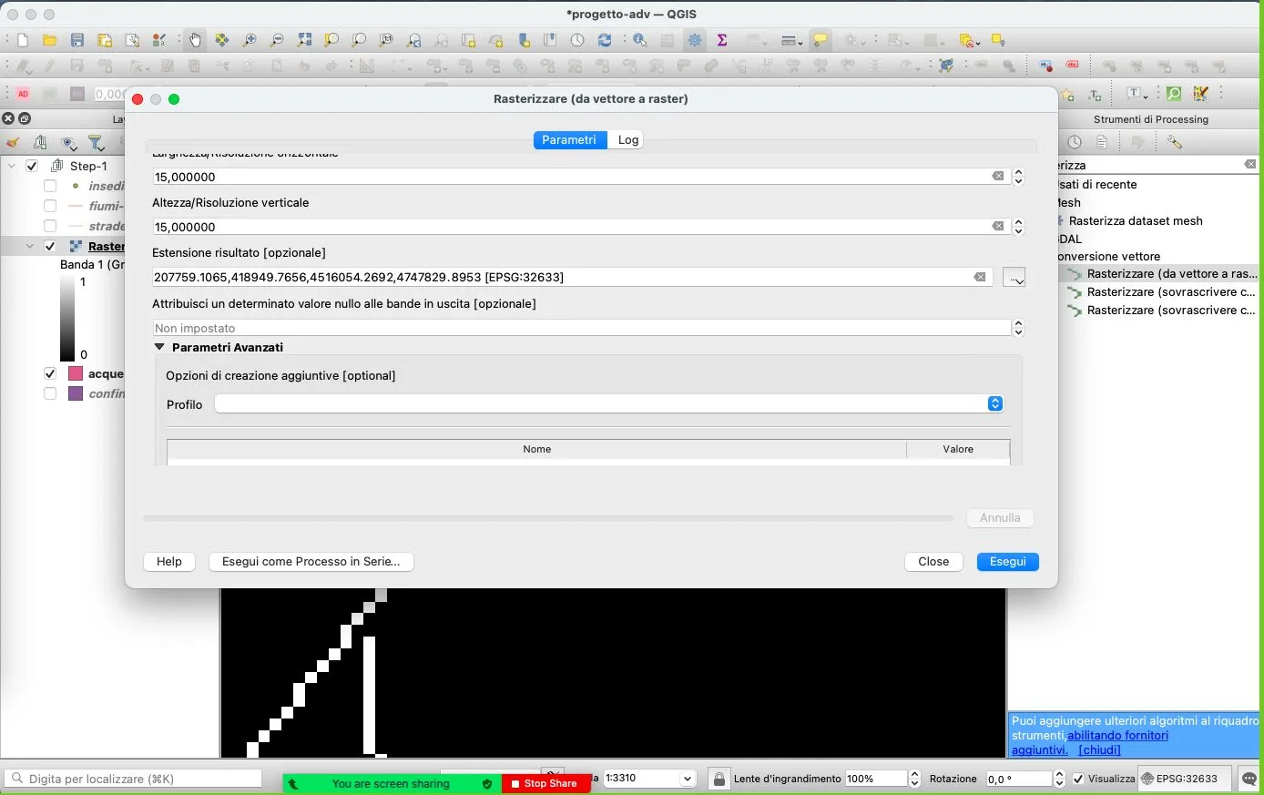
At this point, the operations described above can be repeated, with the same parameters, for all the other available layers, namely:
fiumi-lazio,acque-interne-lazio, andinsediamenti-imperialiThe only exception concerns the resolution of the last item,insediamenti-imperiali, for which we can use an output resolution of 30x30m (Width/Horizontal resolution:30,000000andHeight/Vertical resolution:30,000000).
Finally, a second layer group called Step-2 can be created, and all the rasters created in the previous steps moved into it.
2. Creating a single hydrographic data layer
At present, the hydrographic information is spread across two different rasters, namely fiumi-lazio and acque-interne-lazio. To proceed with the analysis it is useful to merge this information into a single file, and for this we can use a very powerful QGIS tool called the Raster Calculator. As the name suggests, this tool works like a calculator, performing mathematical operations on input data — in this case raster data, which, as is well known, is made up of atomic elements called pixels, each of which is associated with one or more numeric values describing colour or other phenomena, e.g. elevation in the case of DEMs.
- Search for and open
Raster Calculatorin the processing panel (underGDAL>Raster miscellaneous) - Enter the expression:
"acque-interne-raster@1" + "fiumi-raster@1" - Use
confine-rasteras theReference layer(s) - Save the file as
idrografia-3-valori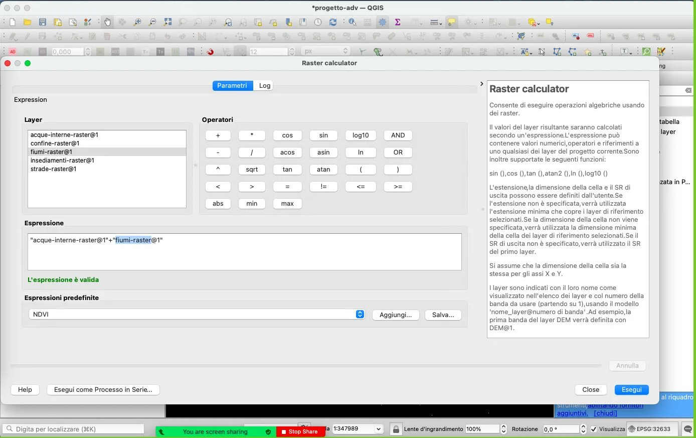
The expression entered, "acque-interne-raster@1" + "fiumi-raster@1", denotes a simple addition between the values of the individual pixels of each layer that occupy the same geographic space (i.e. that overlap). Note that here we are giving a precise indication of which band to use for each raster, through the @1 suffix, even though these particular rasters have only one band. Other, more complex types of raster can have 3 or more bands. This is the case with RGB images, which have 3 bands (or channels), so that image@1 refers to the red values (band 1), image@2 to the green band values, and image@3 to the blue values. This feature becomes much more interesting in the case of multi- or hyperspectral images, where the number of bands can be very high indeed.
The output raster, namely raster_idrografia, will have a value of 1 in pixels where a watercourse is present.
Important: areas where both watercourses (rivers) and lakes are found, however, will have a value of 2. To correct this and bring all areas with lakes and rivers back to a value of 1, follow the next step:
- Eliminate the value 2 and replace it with 1 in the
idrografia-3-valorilayer- Open the
Raster Calculatoragain - Use the following expression:
"idrografia-3-valori@1" > 0 - Save the file as
idrografia-raster
- Open the
- Create a layer group called
Step-3and include in it all the rasters created in this step - Proximity analysis (raster distance)
- Open the
Proximity (Raster Distance)tool (underGDAL>Raster analysis) - Under
Input layerselectstrade-raster - Set
Distance unitstoGeoreferenced units - Set
Maximum distance to be generatedto6000(= 6km) - Set
NoData valuetoNot set - Save the file as
strade-prossimita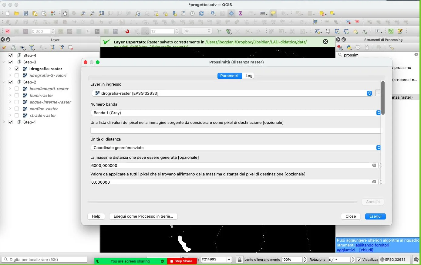
- Open the
Layer Stylingpanel - In
Color ramp, set the maximum value (max) to6000 - Repeat the same operations for the
idrografia-rasterandinsediamenti-rasterlayers
- Open the
- Reclassifying roads, defining three classes, respectively:
- 100, which covers areas up to 1km away,
- 50, which covers areas between 1km and 5km, and
- 10, which covers areas more than 6km away.
- Open the
Raster Calculator - Enter the following expression:
100*("strade-prossimita@1"<=1000) + 50*("strade-prossimita@1">1000)*("strade-prossimita@1"<=6000) + 10*("strade-prossimita@1">6000) - In
Reference layer(s)selectconfine-lazio - Save the file as
strade-riclassificato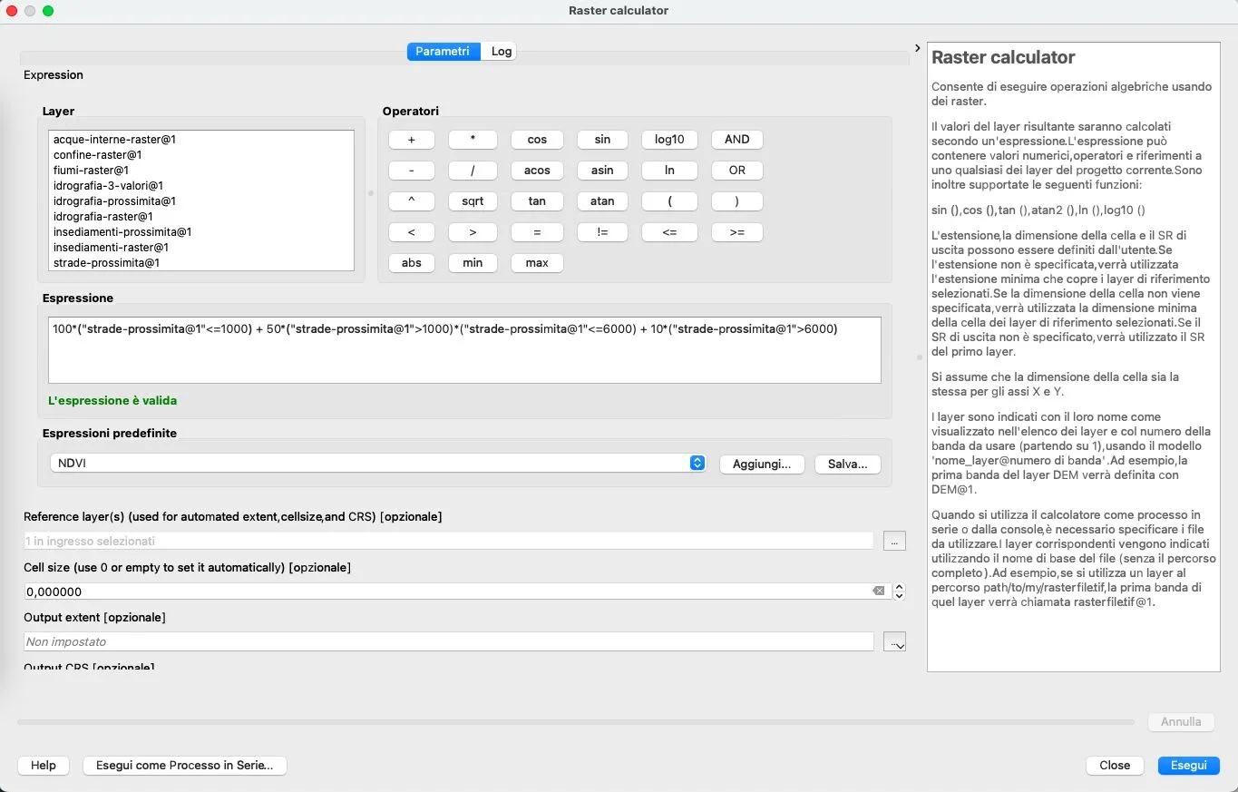
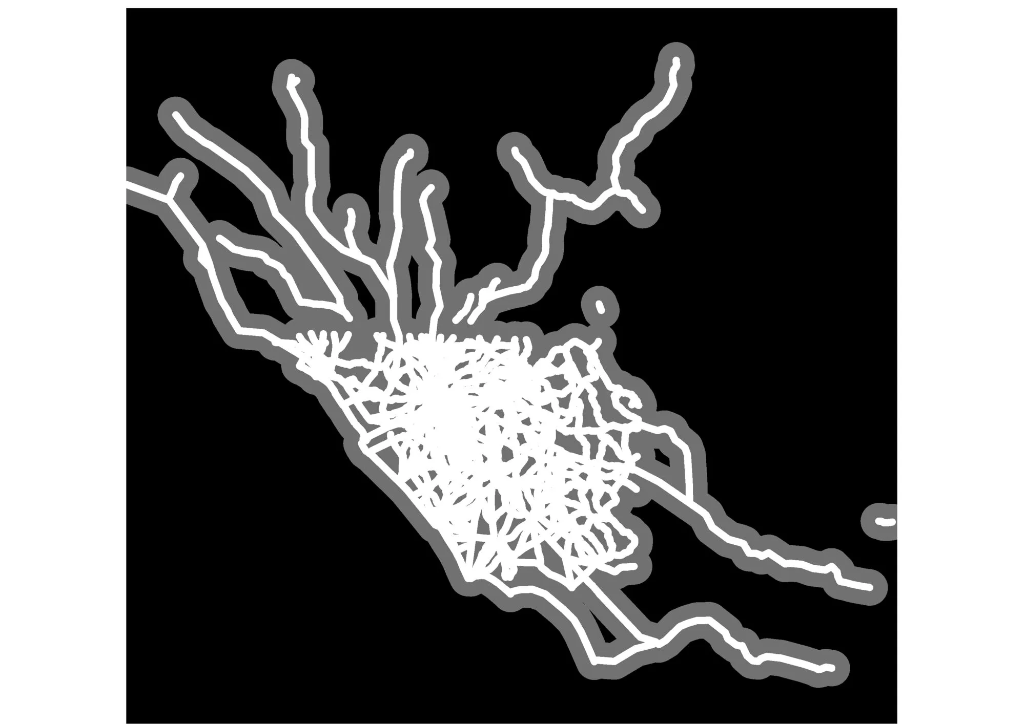
The expression 100*("strade-prossimita@1"<=1000) + 50*("strade-prossimita@1">1000)*("strade-prossimita@1"<=6000) + 10*("strade-prossimita@1">6000) deserves a bit of attention and needs some explanation to be understood, as it mixes arithmetic and boolean logic. In particular, the expressions in parentheses ("strade-prossimita@1"<=1000, "strade-prossimita@1">1000 and "strade-prossimita@1"<=6000) are boolean expressions whose output can be either 0 (if false) or 1 (if true). An example will make this even clearer:
- if a pixel has the value
4524, then"strade-prossimita@1"<=1000returns 0;"strade-prossimita@1">1000returns 1;"strade-prossimita@1"<=6000returns 1;"strade-prossimita@1">6000returns 0; We therefore obtain the expression100*0 + 50*1*1 + 10*0, which results in0+50+0, that is50.
Water
Similarly to the roads, we can now reclassify the water features as well, again defining three classes, chosen arbitrarily. Unlike roads, which are an attracting element, hydrography is a repelling element, so the highest score will be given to the most remote distances, respectively:
- 100, which covers the areas (pixels) located more than 6km away from a hydrographic feature,
- 50, which covers areas between 1km and 5km, and
- 10, which covers areas less than 1km away.
An exercise you can try on your own is to treat distance from water as an ambivalent factor, where being too close should be a penalty, exactly like being too far away, giving the highest score to an intermediate distance.
The procedure is as follows:
- Open the
Raster Calculator - Enter the following expression:
100*("idrografia-prossimita@1">6000) + 50*("idrografia-prossimita@1">1000) * ("idrografia-prossimita@1"<=6000) + 10*("idrografia-prossimita@1"<1000) - In
Reference layer(s)selectconfine-lazio - Save the file as
idrografia-riclassificato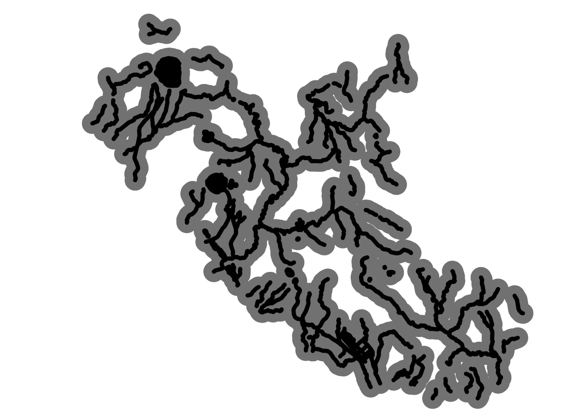
Settlements
Finally, let’s also reclassify the settlements, defining three classes, respectively:
- 100, which covers areas more than 6km away,
- 50, which covers areas between 1km and 5km, and
- 10, which covers areas less than 1km away.
- Open the
Raster Calculator - Enter the following expression:
100*("insediamenti-prossimita@1">6000) + 50*("insediamenti-prossimita@1">1000) * ("insediamenti-prossimita@1"<=6000) + 10*("insediamenti-prossimita@1"<1000) - In
Reference layer(s)selectconfine-lazio - Save the file as
insediamenti-riclassificato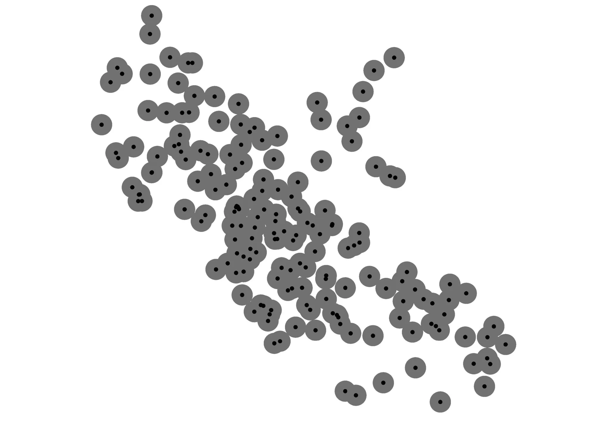
5. Combining the results
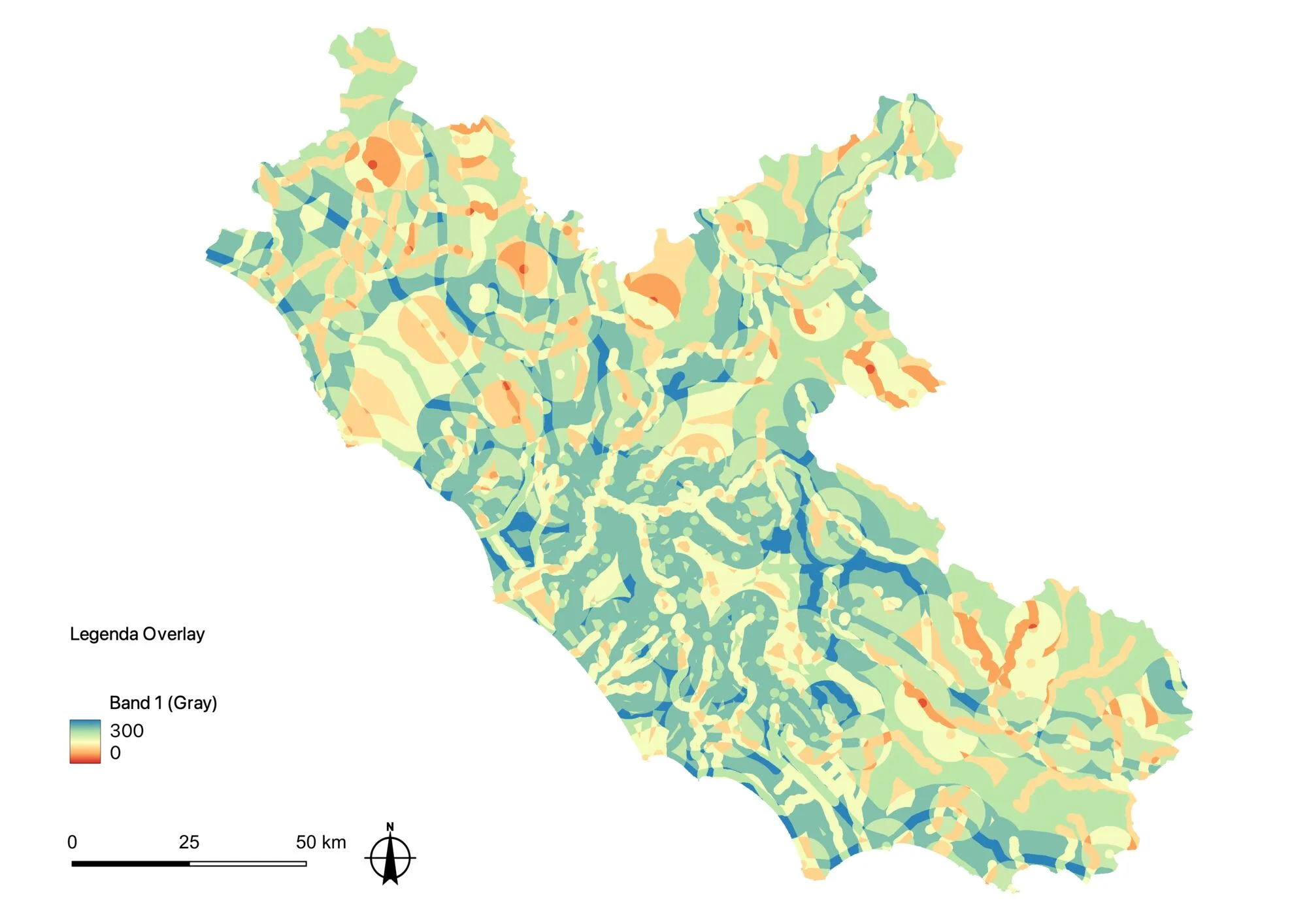
At this point we have everything we need to proceed with the multi-criteria overlay analysis, in which all the reclassified rasters will be summed using the Raster Calculator tool, in order to obtain a single output that answers the question originally posed:
“Which areas of the present-day Lazio region present optimal characteristics for the development of Roman imperial-period settlements, but which, to date, have not yielded reliable traces in this sense?”
The procedure is as follows
- Open the
Raster Calculator - Enter the following expression:
("strade-riclassificato@1" + "idrografia-riclassificato@1" + "insediamenti-riclassificato@1" ) * "confine-raster@1" - In
Reference layer(s)selectconfine-lazio - Save the file as
overlay
The sum expression needs a brief explanation.
- The last operation on the right, multiplying by
"confine-raster@1", ensures that all values located outside the regional boundary become0, since they are multiplied by0; the others remain unchanged, since they are multiplied by1.
6. Assigning a more explanatory symbology
The pixel values of the final raster called overlay can range from 0 to 300, where 0 is the area considered least optimal for the development of Roman imperial-period settlements in Lazio, while 300 is the one considered most suitable. To best visualize the result of the analysis, we can assign a symbology that applies a colour gradient scale to the overlay raster and that, above all, makes it possible to best represent the shades of variation between the values 0 and 300.
The procedure is as follows:
- Open the layer’s properties
- Under
Render typesetSingleband pseudocolor - Classify
Final note
As we have seen in steps 4 and 5, several conventions are being adopted for classifying the data. For example, the decision to divide everything into three classes, and the weights, in numerical terms, given to each class.
The decision to give all classes equal weight in step 5 is likewise arbitrary. One possible refinement could be to give different weights to proximity to existing sites, hydrography, and the road network, with the latter possibly being multiplied by a coefficient.
But from here on, it becomes a matter of proceeding with the interpretation of the data, from a strictly archaeological point of view!
Online sources
- Ancient World Mapping Center, http://awmc.unc.edu/wordpress/, last accessed on 25 October 2022.
- DIVA-GIS: free, simple & effective, https://www.diva-gis.org/gdata, last accessed on 25 October 2022.
- OpenTopography: High-Resolution Topography Data and Tools, https://www.opentopography.org/, last accessed on 25 October 2022.
- Pleiades, https://pleiades.stoa.org/, last accessed on 25 October 2022.
- QGIS Tutorials and Tips, http://www.qgistutorials.com/it/docs/3/multi_criteria_overlay.html, last accessed on 25 October 2022.