Exporting sections and elevations from Agisoft Metashape models

The increasingly widespread use of archaeological survey methods based on photogrammetry makes it necessary to develop procedures that allow “traditional products” of archaeological documentation to be recovered from 3D models. While the creation of plans is natively handled by specialized software, such as the extremely popular Agisoft Metashape, producing elevations and sections requires extra work.

Introduction

The aim of this article is to provide a practical guide for extracting orthophotos of vertical surfaces, such as sections or elevations, from a three-dimensional photogrammetric survey. At the end of the process, the result will therefore be a two-dimensional image, metrically correct and free of perspective distortion, and ideally of excellent quality, although the resolution will of course depend on the quality of the original survey. This image can be used as an element for publications or as a raster base for creating digital surveys in a GIS environment (see https://lad.saras.uniroma1.it/blog/statistiche-metrologiche-automatiche-con-qgis/ for some of the potential of these applications).

In this tutorial, we will use, by way of example, some data collected as part of the Archaeological Mission to Çuka e Ajtoit (Albania), and specifically a photogrammetric survey obtained through rendering and digital overlapping of photographs taken by drone. The steps needed to obtain such a survey will not be detailed here. The result we will obtain is an orthophoto of the surviving elevation of a wall built in polygonal masonry. Although the methodology used can be considered universally valid, the commands given here refer specifically to the Agisoft Metashape software, one of the most widely used tools in our field thanks to its excellent balance of quality, ease of use and price.

Agisoft Metashape makes it extremely easy to create orthomosaics and other products, such as DEMs, from three-dimensional models, following a straightforward workflow when projecting onto a plane that runs horizontally (the XY plane). It is nevertheless possible to use a projection plane other than the ‘geographic’ one, and among the various options, one of the most flexible for us archaeologists is the one that lets you define a plane by providing three points — three coordinate triplets. These are equivalent to the traditional ‘string line’ we use in the field to define the projection plane, normally defined by two points (the two pegs), while the third dimension of the plane is given by the plumb line. This article aims to define a quick and precise method for defining a vertical projection plane inside Metashape.

Step 1: ‘Setting the string line’

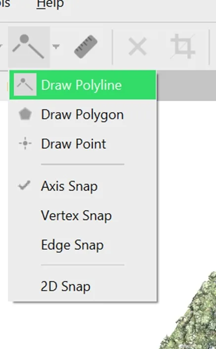
As with the most classic direct survey, the first operation to perform will be to establish the horizontal reference plane using a ‘string line’, digitally replaced by a linear element with elevation values (a linestringZ). To produce the line in Agisoft Metashape, you will first need to activate the Draw Polyline command from the Toolbar (see image) or from the Model drop-down menu.

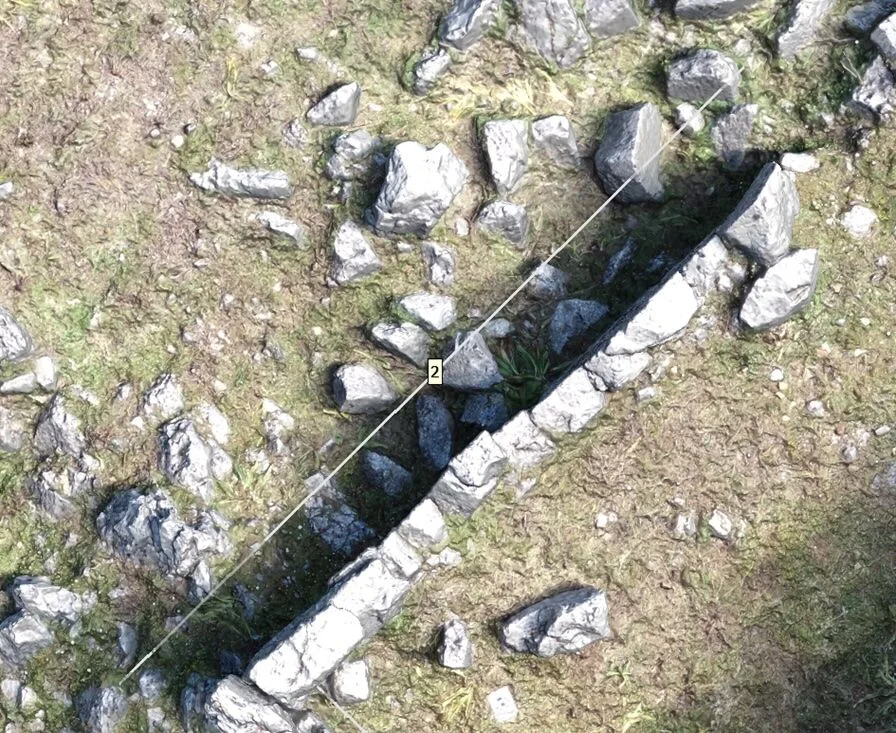
Once the option is selected, you will need to trace the reference line, taking care to place the start and end points of the geometry at an appropriate distance from the element to be surveyed (the facade) and to exclude, as far as possible, any ‘intruding’ elements in elevation that might come between it and our simulated viewpoint (see image below). Once you have finished drawing the geometry, give it an easily recognizable name and save. For now we do not need to worry about the third dimension, and we only need to make sure our line (the ‘string line’) is as parallel as possible to the surface to be represented. Finally, it is good practice to give the line a meaningful name, in case we need to extract many elevations from our model, e.g. prosp_1, prosp_2, etc.

Step 2: Exporting and normalizing the coordinates

Once the geometry has been created, you can extract all the related data — which, in our case, will be the coordinates of the two endpoints and the name entered when it was created — in GeoJSON format, through the menu File > Export > Export shapes.

GeoJSON is a vector-element encoding format that uses plain text, so the resulting file can be opened with any text document reader. On Windows, it is recommended not to use the Notepad program that comes with the operating system, as it may introduce problems with the encoding of certain characters, such as line breaks. For this reason, the use of Notepad++, Notepad2, and similar programs is recommended. This will make it possible to view and edit the attributes of the line we have just created by displaying the geometries as text. Naturally, this operation will export all elements belonging to the Shapes category present in our project, grouping them into a Feature collection. The result will therefore look something like this:

1
{
2
  "features": [
3
    {
4
      "geometry": {
5
        "coordinates": [
6
          [
7
            20.119747561405298,
8
            39.682003256417353,
9
            183.32642292420428
10
          ],
11
          [
12
            20.119615235830111,
13
            39.681909476672189,
14
            185.07040807192504
15
          ]
16
        ],
17
        "type": "LineString"
18
      },
19
      "properties": {
20
        "LAYER": "Layer",
21
        "NAME": "prosp_1"
22
      },
23
      "type": "Feature"
24
    },
25
    {
26
      "geometry": {
27
        "coordinates": [
28
          [
29
            20.119487453675205,
30
            39.681834231537692,
31
            184.37274330360373
32
          ],
33
          [
34
            20.119425195388814,
35
            39.68179554340319,
36
            182.49861374549914
37
          ],
38
          [
39
            20.119425195388814,
40
            39.68179554340319,
41
            182.49861374549914
42
          ]
43
        ],
44
        "type": "LineString"
45
      },
46
      "properties": {
47
        "LAYER": "Layer",
48
        "NAME": "prosp_2"
49
      },
50
      "type": "Feature"
51
    },
52
  ],
53
  "type": "FeatureCollection"
54
}

It will now be necessary to isolate and ‘clean up’ the data, keeping only that of the line (or lines) we are interested in extracting. In the example above, we included a line mistakenly created with 3 points, so as to also introduce the solution to this possible source of error. The first step will be to identify and isolate the line we are interested in through the name assigned to it when it was created (in the example, ‘prosp_2’), to be found at the end of the element’s attributes. We can then proceed with a digital ‘cleanup’ of the data, first removing everything not relevant to the line we are interested in, and then the values of our line that we are not interested in keeping. In the case of the ‘prosp_2’ line, among the elements to be removed was also the ‘middle’ point, which we have no interest in processing. The result at this point in the process will therefore look like this:

1
[
2
  [
3
    20.119697765107098,
4
    39.681844866941844,
5
    188.21852672754807
6
  ],
7
  [
8
    20.119875100191919,
9
    39.681977508049947,
10
    187.15508159538413
11
  ]
12
]

We have thus isolated the x, y and z values of the two endpoints of the line (our ‘string line’). The next step will consist of removing the brackets, isolating the values of the two points on separate lines and, finally, changing the elevation value to a more practical standard value than the real one. For the purposes of our work, it does not matter whether the elevation value is below the walking surface, but it is worth making sure it does not exceed the base of the element to be surveyed. After these steps, the result should look similar to the following:

1
20.119697765107098,39.681844866941844,186.5
2
20.119615235830107,39.681909476672189,186.5

Note: the format above is known as CSV (comma-separated values), an extremely simple (but powerful) way of structuring tabular data as text. Each line corresponds to a record and commas separate the columns. A CSV file can be opened with any text editor (the same caveat given above for Notepad on Windows applies) but also with spreadsheet programs such as LibreOffice Calc or Apache OpenOffice Calc. Once again, it is not advisable to open and edit CSV files with Microsoft Excel, since this program automatically formats our data in unwanted ways, also causing loss of information.

We now have the references for the horizontal plane (our digital ‘string line’). For the task at hand, however, we still need to create a third reference for the vertical axis. To do this, it is enough to duplicate the data of one of the horizontal references, increasing the value of the Z parameter. Naturally, the new elevation must also be higher than that of the element to be surveyed, if we want to avoid the result being ‘cut off’ during rendering. Finally, let’s assign names to each individual point. The names are not binding, but keep in mind that they will remain as such in the Metashape project, so it is advisable to use simple naming for better management, one that refers back to the name of the original line. We will give meaningful names to make our life easier in Metashape, so 2-o stands for the origin point of the projection plane for elevation 2; 2-x stands for the point defining the x-axis of the projection plane for elevation 2; 2-y stands for the point defining the y-axis of elevation 2.
The x and y coordinates of point 2-y are identical to those of point 2-o (we can use copy/paste to create the line), differing only in the y coordinate, which we have arbitrarily increased, rounding it to 190. It is not important to define a specific value, but simply to give a direction, increasing the y coordinate of the origin point (2-o) by even a very small amount.

1
2-o,20.119697765107098,39.681844866941844,186.5
2
2-x,20.119615235830107,39.681909476672189,186.5
3
2-y,20.119697765107098,39.681844866941844,190

In this tutorial, for the sake of example, we have proposed the simple extraction of data from a single line for producing a single elevation. However, if, as is often the case, our goal is to extract a series of elevations, then the steps listed in paragraphs 1–3 can all be carried out simultaneously. If that were our goal, it would in fact be enough to isolate all the points we are interested in from the GeoJSON file, again on separate lines, in order to perform a single import into Metashape. Using the example given in figure 3 as a basis, the result produced would be as follows:

1
1-o,20.119747561405298,39.682003256417353,182.5
2
1-x,20.119615235830111,39.681909476672189,182.5
3
1-t,20.119747561405298,39.682003256417353,188
4
2-o,20. 119697765107098,39.681844866941844,186.5
5
2-x,20. 119615235830107,39.681909476672189,186.5
6
2-y, 20. 119697765107098,39.681844866941844,190
7
3-o,20.119487453675205,39.681834231537692,182
8
3-x,20.119425195388814,39.68179554340319,182
9
3-y,20.119487453675205,39.681834231537692,186
10
4-o,20.119432266860173,39.681794354576304,182
11
4-x,20.11947527028088,39.681755063212833,182
12
4-y,20.119432266860173,39.681794354576304,186

Step 3: importing the CSV file

Now that we have the three points to which we will anchor the reference axes, and have organized them in CSV format, the next step will be to import them into our project. To do this, simply use Metashape’s File > Import > Import Reference command. Before performing the operation, it will be important to make sure that the coordinate system, the column delimiter character (in our case the comma), and the selected starting row are set correctly.

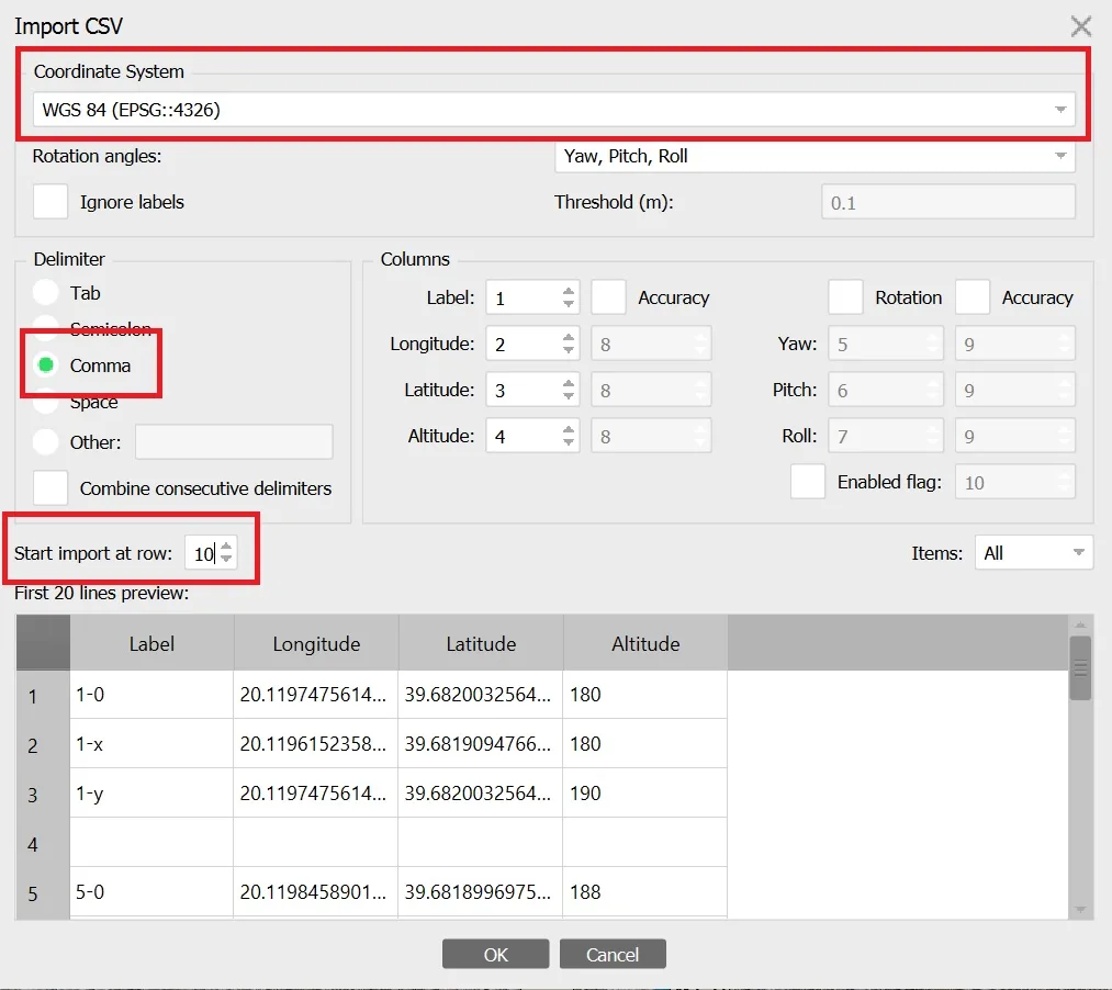
Once these precautions have been taken, you can perform the operation and, in the window that follows, you will be asked to create new markers whose names will correspond to the first value identified for each element (in the example in the previous paragraph, 2-o, 2-x and 2-y). Once this further request is approved, the markers will be available in our project. Once the operation has been carried out, we can make sure the markers have been placed in the correct position by enabling their display through the Model > Show/Hide Items > Show Markers command.

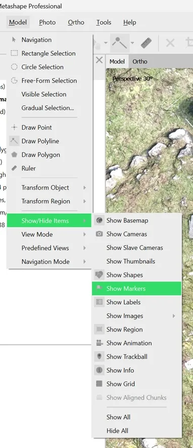
WARNING: if markers with the same name as the incoming ones are already present in the project, the system will overwrite the data for those markers.

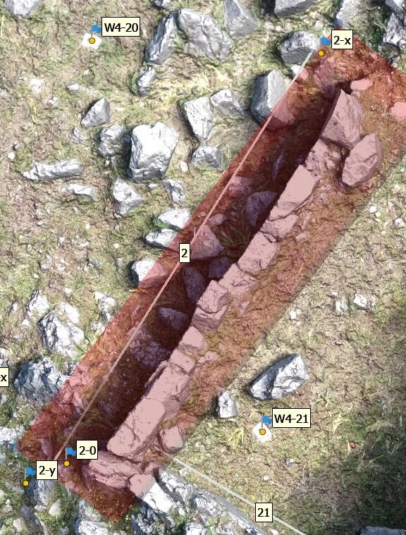
Step 4: Extracting the orthomosaic of the elevation

Now, only the last preliminary operation remains before proceeding to extract our orthophoto. To reduce processing time and avoid exporting elements unrelated to what we are interested in obtaining, we need to resize the region of interest using the Move Region command from the Toolbar or from the Model > Transform Region > Move region menu item. The region of interest should be narrowed as much as possible around the image to be exported, while making sure it fully encloses all the relevant elements. Since this is three-dimensional work, remember to make sure the region of interest encloses the element to be surveyed not only in length and width, but also in height.

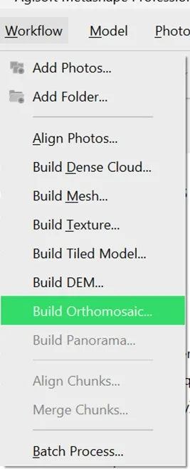
With this last preliminary operation complete, we can finally proceed to export the orthophoto. To do this, let’s open the Build orthomosaic panel from the Workflow menu item:

Here, we choose a planar-type projection and set as reference the markers entered in the previous step, taking care to enter them correctly. In the example given in the previous steps, points 2-o and 2-x will serve as the reference for the horizontal axis, while 2-o and 2-y will define the vertical one:

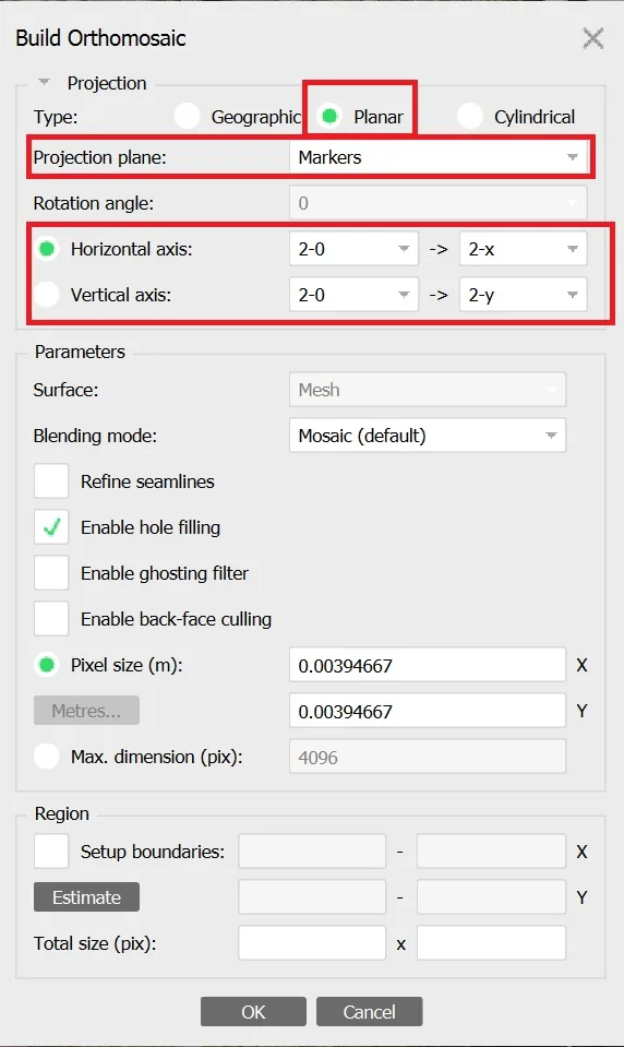
Once these operations have been carried out, we can proceed to create our orthomosaic, which will then be inserted into the project.

WARNING: the orthophoto will be inserted into the project as ‘Orthomosaic’, overwriting any previous element with that name. In cases where you intend to export multiple elements, you will therefore first need to export the work in TIFF format (next step), and only afterwards will you be able to create the next orthomosaic, which will overwrite the one currently present in the project.

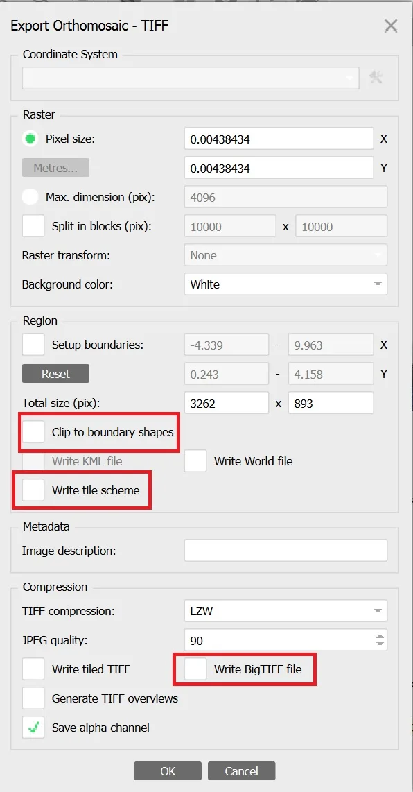
Once the final result has been checked within Metashape, we can finally proceed to export the two-dimensional image in TIFF format, by right-clicking on the orthomosaic entry in the Workspace panel and selecting Export Orthomosaic. Once the image name and destination folder have been selected, the export settings panel will open. It is recommended to pay attention to the Clip to boundary shapes and Write Tile Scheme options, which, for the purposes of this tutorial, should both be unchecked, as shown in the image. If the export results in an empty file, it has sometimes helped to also uncheck the ‘Write BigTIFF file’ setting, which we nevertheless recommend keeping enabled if this problem does not occur.

Once the orthomosaic export operation is complete — which can take a very long time (several hours, if the three-dimensional model is high-resolution, the area to be exported is very large, and the machine performing the calculation is not particularly powerful) — we will finally have the elevation drawing of our facade in TIFF format.